Recursion (computer science)
From Wikipedia, the free encyclopedia
Recursion in computer science is a way of thinking about and solving problems. In fact, recursion is one of the central ideas of computer science. [1] Solving a problem using recursion means the solution depends on solutions to smaller instances of the same problem. [2]
"The power of recursion evidently lies in the possibility of defining an infinite set of objects by a finite statement. In the same manner, an infinite number of computations can be described by a finite recursive program, even if this program contains no explicit repetitions." [3]
Most high-level computer programming languages support recursion by allowing a function to call itself within the program text. Imperative languages define looping constructs like “while” and “for” loops that are used to perform repetitive actions. Some functional programming languages do not define any looping constructs but rely solely on recursion to repeatedly call code. Computability theory has proven that these recursive only languages are mathematically equivalent to the imperative languages, meaning they can solve the same kinds of problems even without the typical control structures like “while” and “for”.

Contents |
[edit] Recursive algorithms
A common method of simplification is to divide a problem into sub-problems of the same type. This is known as dialecting. As a computer programming technique, this is called divide and conquer, and it is key to the design of many important algorithms, as well as a fundamental part of dynamic programming.
Virtually all programming languages in use today allow the direct specification of recursive functions and procedures. When such a function is called, the computer (for most languages on most stack-based architectures) or the language implementation keeps track of the various instances of the function (on many architectures, by using a call stack, although other methods may be used). Conversely, every recursive function can be transformed into an iterative function by using a stack.
Most (but not all) functions and procedures that can be evaluated by a computer can be expressed in terms of a recursive function (without having to use pure iteration),[citation needed] in continuation-passing style; conversely any recursive function can be expressed in terms of (pure) iteration, since recursion in itself is iterative too.[citation needed] In order to evaluate a function by means of recursion, it has to be defined as a function of itself (e.g. the factorial n! = n * (n - 1)! , where 0! is defined as 1). Clearly thus, not all function evaluations lend themselves to a recursive approach. In general, all non-infinite functions can be described recursively directly; infinite functions (e.g. the series for e = 1/1! + 2/2! + 3/3!...) need an extra 'stopping criterion', e.g. the number of iterations, or the number of significant digits, because otherwise recursive iteration would result in an endless loop.
To give a very literal example of this: If an unknown word is seen in a book, the reader can make a note of the current page number and put the note on a stack (which is empty so far). The reader can then look the new word up and, while reading on the subject, may find yet another unknown word. The page number of this word is also written down and put on top of the stack. At some point an article is read that does not require any explanation. The reader then returns to the previous page number and continues reading from there. This is repeated, sequentially removing the topmost note from the stack. Finally, the reader returns to the original book. This is a recursive approach.
Some languages designed for logic programming and functional programming provide recursion as the only means of repetition directly available to the programmer. Such languages generally make tail recursion as efficient as iteration, letting programmers express other repetition structures (such as Scheme's map and for) in terms of recursion.
Recursion is deeply embedded in the theory of computation, with the theoretical equivalence of μ-recursive functions and Turing machines at the foundation of ideas about the universality of the modern computer.
[edit] Recursive programming
Creating a recursive procedure essentially requires defining a "base case", and then defining rules to break down more complex cases into the base case. Key to a recursive procedure is that with each recursive call, the problem domain must be reduced in such a way that eventually the base case is arrived at.
Some authors classify recursion as either "generative" or "structural". The distinction is made based on where the procedure gets the data that it works on. If the data comes from a data structure like a list, then the procedure is "structurally recursive"; otherwise, it is "generatively recursive".[4]
Many well-known recursive algorithms generate an entirely new piece of data from the given data and recur on it. HTDP (How To Design Programs) refers to this kind as generative recursion. Examples of generative recursion include: gcd, quicksort, binary search, mergesort, Newton's method, fractals, and adaptive integration.[5]
[edit] Recursive procedures (generative recursion)
[edit] Factorial
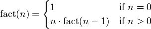
A classic example of a recursive procedure is the function used to calculate the factorial of an integer.
Function definition:
| Pseudocode (recursive): |
|---|
function factorial is: |
A recurrence relation is an equation that relates later terms in the sequence to earlier terms[6].
Recurrence relation for factorial:
- bn = nbn − 1
- b0 = 1
| Computing the recurrence relation for n = 4: |
|---|
b4 = 4 * b3 |
This factorial function can also be described without using recursion by making use of the typical looping constructs found in imperative programming languages:
| Pseudocode (iterative): |
|---|
function factorial is: |
Scheme, however, is a functional programming language and does not define any looping constructs. It relies solely upon recursion to perform all looping. Because Scheme is tail-recursive, a recursive procedure can be defined that implements the factorial procedure as an iterative process — meaning that it uses constant space but linear time.
[edit] Fibonacci
Another well known recursive sequence is the Fibonacci numbers. The first few elements of this sequence are: 0, 1, 1, 2, 3, 5, 8, 13, 21...
Function definition: 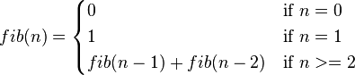
| Pseudocode |
|---|
function fib is: input: integer n such that n >= 0 |
Recurrence relation for Fibonacci:
bn = bn-1 + bn-2
b1 = 1, b0 = 0
| Computing the recurrence relation for n = 4: |
|---|
  b4            = b3 + b2
                = b2 + b1 + b1 + b0
                = b1 + b0 + 1 + 1 + 0
                = 1 + 0 + 1 + 1 + 0
                = 3
|
This Fibonacci algorithm is especially bad because each time the function is executed, it will make two function calls to itself each of which in turn makes two more function calls and so on until they "bottom out" at 1 or 0. This is an example of "tree recursion", and grows exponentially in time and linearly in space requirements.[7]
[edit] Greatest common divisor
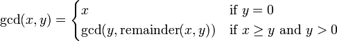
Another famous recursive function is the Euclidean algorithm, used to compute the greatest common divisor of two integers. Function definition:
| Pseudocode (recursive): |
|---|
function gcd is: input: integer x, integer y such that x >= y and y > 0 |
Recurrence relation for greatest common divisor, where x%y expresses the remainder of x / y:
- gcd(x,y) = gcd(y,x%y)
- gcd(x,0) = x
| Computing the recurrence relation for x = 27 and y = 9: |
|---|
gcd(27, 9)   = gcd(9, 27 % 9)
             = gcd(9, 0)
             = 9
|
| Computing the recurrence relation for x = 259 and y = 111: |
gcd(259, 111)   = gcd(111, 259 % 111)
                = gcd(111, 37)
                = gcd(37, 0)
                = 37
|
Notice that the "recursive" algorithm above is in fact merely tail-recursive, which means it is equivalent to an iterative algorithm. Below is the same algorithm using explicit iteration. It does not accumulate a chain of deferred operations; rather, its state is maintained entirely in the variables x and y. Its "number of steps grows the as the logarithm of the numbers involved."[8]
| Pseudocode (iterative): |
|---|
function gcd is: |
The iterative algorithm requires a temporary variable, and even given knowledge of the Euclidean algorithm it is more difficult to understand the process by simple inspection, although the two algorithms are very similar in their steps.
[edit] Towers of Hanoi
For a full discussion of this problem's description, history and solution see the main article or one of the many references.[9] [10] Simply put the problem is this: given three pegs, one with a set of N disks of increasing size, determine the minimum (optimal) number of steps it takes to move all the disks from their initial position to another peg without placing a larger disk on top of a smaller one.
Function definition:

Recurrence relation for hanoi:
- hn = 2hn − 1 + 1
- h1 = 1
| Computing the recurrence relation for n = 4: |
|---|
hanoi(4)     = 2*hanoi(3) + 1
             = 2*(2*hanoi(2) + 1) + 1
             = 2*(2*(2*hanoi(1) + 1) + 1) + 1
             = 2*(2*(2*1 + 1) + 1) + 1
             = 2*(2*(3) + 1) + 1
             = 2*(7) + 1
             = 15
|
Example Implementations:
| Pseudocode (recursive): |
|---|
function hanoi is: |
Although not all recursive functions have an explicit solution, the Tower of Hanoi sequence can be reduced to an explicit formula. [11]
| An explicit formula for Towers of Hanoi: |
|---|
h1 = 1   = 21 - 1
h2 = 3   = 22 - 1
h3 = 7   = 23 - 1
h4 = 15  = 24 - 1
h5 = 31  = 25 - 1
h6 = 63  = 26 - 1
h7 = 127 = 27 - 1
In general: hn = 2n - 1, for all n >= 1 |
[edit] Binary search
The binary search algorithm is a method of searching an ordered array for a single element by cutting the array in half with each pass. The trick is to pick a midpoint near the center of the array, compare the data at that point with the data being searched and then responding to one of three possible conditions: the data is found, the data at the midpoint is greater than the data being searched for, or the data at the midpoint is less than the data being searched for.
Recursion is used in this algorithm because with each pass a new array is created by cutting the old one in half. The binary search procedure is then called recursively, this time on the new (and smaller) array. Typically the array's size is adjusted by manipulating a beginning and ending index. The algorithm exhibits a logarithmic order of growth because it essentially divides the problem domain in half with each pass.
Example Implementation of Binary Search:
 /*
  Call binary_search with proper initial conditions.

  INPUT:
    data is a array of integers SORTED in ASCENDING order,
    toFind is the integer to search for,
    count is the total number of elements in the array

  OUTPUT:
    result of binary_search

 */
 int search(int *data, int toFind, int count)
 {
    //  Start = 0 (beginning index)
    //  End = count - 1 (top index)
    return binary_search(data, toFind, 0, count-1);
 }

 /*
   Binary Search Algorithm.

   INPUT:
        data is a array of integers SORTED in ASCENDING order,
        toFind is the integer to search for,
        start is the minimum array index,
        end is the maximum array index
   OUTPUT:
        position of the integer toFind within array data,
        -1 if not found
 */
 int binary_search(int *data, int toFind, int start, int end)
 {
    //Get the midpoint.
    int mid = start + (end - start)/2;   //Integer division

    //Stop condition.
    if (start > end)
       return -1;
    else if (data[mid] == toFind)        //Found?
       return mid;
    else if (data[mid] > toFind)         //Data is greater than toFind, search lower half
       return binary_search(data, toFind, start, mid-1);
    else                                 //Data is less than toFind, search upper half
       return binary_search(data, toFind, mid+1, end);
 }
[edit] Recursive data structures (structural recursion)
An important application of recursion in computer science is in defining dynamic data structures such as Lists and Trees. Recursive data structures can dynamically grow to a theoretically infinite size in response to runtime requirements; in contrast, a static array's size requirements must be set at compile time.
"Recursive algorithms are particularly appropriate when the underlying problem or the data to be treated are defined in recursive terms." [12]
The examples in this section illustrate what is known as "structural recursion". This term refers to the fact that the recursive procedures are acting on data that is defined recursively.
As long as a programmer derives the template from a data definition, functions employ structural recursion. That is, the recursions in a function's body consume some immediate piece of a given compound value. [13]
[edit] Linked lists
Below is a simple definition of a linked list node. Notice especially how the node is defined in terms of itself. The "next" element of struct node is a pointer to a struct node.
struct node
{
  int n;              // some data
  struct node *next;  // pointer to another struct node
};

// LIST is simply a synonym for struct node * (aka syntactic sugar).
typedef struct node *LIST;
Procedures that operate on the LIST data structure can be implemented naturally as a recursive procedure because the data structure it operates on (LIST) is defined recursively. The printList procedure defined below walks down the list until the list is empty (NULL), for each node it prints the data element (an integer). In the C implementation, the list remains unchanged by the printList procedure.
void printList(LIST lst)
{
    if (!isEmpty(lst))         // base case
    {
       printf("%d ", lst->n);  // print integer followed by a space
       printList(lst->next);   // recursive call
    }
}
[edit] Binary trees
Below is a simple definition for a binary tree node. Like the node for Linked Lists, it is defined in terms of itself (recursively). There are two self-referential pointers - left (pointing to the left sub-tree) and right (pointing to the right sub-tree).
struct node
{
  int n;               // some data
  struct node *left;   // pointer to the left subtree
  struct node *right;  // point to the right subtree
};

// TREE is simply a synonym for struct node * (aka syntactic sugar).
typedef struct node *TREE;
Operations on the tree can be implemented using recursion. Note that because there are two self-referencing pointers (left and right), that tree operations will require two recursive calls. For a similar example see the Fibonacci function and explanation above.
void printTree(TREE t) {
        if (!isEmpty(t)) {            // base case
                printTree(t->left);   // go left
                printf("%d ", t->n);  // print the integer followed by a space
                printTree(t->right);  // go right
        }
}
The above example illustrates an in-order traversal of the binary tree. A Binary search tree is a special case of the binary tree where the data elements of each node are in order.
[edit] Recursion versus iteration
In the "factorial" example the iterative implementation is likely to be slightly faster in practice than the recursive one. This is almost definite for the Euclidean Algorithm implementation. This result is typical, because iterative functions do not pay the "function-call overhead" as many times as recursive functions, and that overhead is relatively high in many languages. (Note that an even faster implementation for the factorial function on small integers is to use a lookup table.)
There are other types of problems whose solutions are inherently recursive, because they need to keep track of prior state. One example is tree traversal; others include the Ackermann function and divide-and-conquer algorithms such as Quicksort. All of these algorithms can be implemented iteratively with the help of a stack, but the need for the stack arguably nullifies the advantages of the iterative solution.
Another possible reason for choosing an iterative rather than a recursive algorithm is that in today's programming languages, the stack space available to a thread is often much less than the space available in the heap, and recursive algorithms tend to require more stack space than iterative algorithms. However, see the caveat below regarding the special case of tail recursion.
[edit] Tail-recursive functions
Tail-recursive functions are functions ending in a recursive call that does not build-up any deferred operations. For example, the gcd function (re-shown below) is tail-recursive; however, the factorial function (also re-shown below) is "augmenting recursive" because it builds up deferred operations that must be performed even after the final recursive call completes. With a compiler that automatically optimizes tail-recursive calls, a tail-recursive function such as gcd will execute using constant space. Thus the process it generates is iterative and equivalent to using imperative language control structures like the "for" and "while" loops.
| Tail recursion: | Augmenting recursion: |
|---|---|
//INPUT: Integers x, y such that x >= y and y > 0 int gcd(int x, int y) { if (y == 0) return x; else return gcd(y, x % y); } |
//INPUT: n is an Integer such that n >= 1 int fact(int n) { if (n == 1) return 1; else return n * fact(n - 1); } |
The significance of tail recursion is that when making a tail-recursive call, the caller's return position need not be saved on the call stack; when the recursive call returns, it will branch directly on the previously saved return position. Therefore, on compilers which support tail-recursion optimization, tail recursion saves both space and time.
[edit] Order of function calling
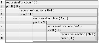
The order of calling a function may change the execution of a function, see this example in C language:
[edit] Function 1
void recursiveFunction(int num) {
   if (num < 5) {
      printf("%d\n", num);
      recursiveFunction(num + 1);
   }
}
[edit] Function 2 with swapped lines
void recursiveFunction(int num) {
   if (num < 5) {
      recursiveFunction(num + 1);
      printf("%d\n", num);
   }
}

[edit] Direct and indirect recursion
Direct recursion is when a function calls itself. Indirect recursion is when (for example) function A calls function B, function B calls function C, and then function C calls function A. Long chains and branches are possible, see Recursive descent parser.
[edit] See also
- Mutual recursion
- Anonymous recursion
- μ-recursive function
- Primitive recursive function
- Functional programming
- Kleene-Rosser paradox
- McCarthy 91 function
- Ackermann function
- Sierpiński curve
[edit] Notes and References
- ^ Epp, Susanna (1995). Discrete Mathematics with Applications (2nd ed.). p. 427.
- ^ Graham, Ronald; Donald Knuth, Oren Patashnik (1990). Concrete Mathematics. Chapter 1: Recurrent Problems. http://www-cs-faculty.stanford.edu/~knuth/gkp.html.
- ^ Wirth, Niklaus (1976). Algorithms + Data Structures = Programs. Prentice-Hall. p. 126.
- ^ Felleisen, Matthias; Robert Bruce Findler, Matthew Flatt, Shriram Krishnamurthi (2001). How to Design Programs: An Introduction to Computing and Programming. Cambridge, MASS: MIT Press. p. art V "Generative Recursion". http://www.htdp.org/2003-09-26/Book/curriculum-Z-H-31.html.
- ^ Felleisen, Matthias (2002), "Developing Interactive Web Programs", in Jeuring, Johan, Advanced Functional Programming: 4th International School, Oxford, UK: Springer, pp. 108.
- ^ Epp, Susanna (1995). Discrete Mathematics with Applications. Brooks-Cole Publishing Company. p. 424.
- ^ Abelson, Harold; Gerald Jay Sussman (1996). Structure and Interpretation of Computer Programs. Section 1.2.2. http://mitpress.mit.edu/sicp/full-text/book/book-Z-H-11.html#%_sec_1.2.2.
- ^ Abelson, Harold; Gerald Jay Sussman (1996). Structure and Interpretation of Computer Programs. Section 1.2.5. http://mitpress.mit.edu/sicp/full-text/book/book-Z-H-11.html#%_sec_1.2.5.
- ^ Graham, Ronald; Donald Knuth, Oren Patashnik (1990). Concrete Mathematics. Chapter 1, Section 1.1: The Tower of Hanoi. http://www-cs-faculty.stanford.edu/~knuth/gkp.html.
- ^ Epp, Susanna (1995). Discrete Mathematics with Applications (2nd ed.). pp. 427–430: The Tower of Hanoi.
- ^ Epp, Susanna (1995). Discrete Mathematics with Applications (2nd ed.). pp. 447–448: An Explicit Formula for the Tower of Hanoi Sequence.
- ^ Wirth, Niklaus (1976). Algorithms + Data Structures = Programs. Prentice-Hall. p. 127.
- ^ Felleisen, Matthias (2002), "Developing Interactive Web Programs", in Jeuring, Johan, Advanced Functional Programming: 4th International School, Oxford, UK: Springer, pp. 108.
[edit] External links
- Harold Abelson and Gerald Sussman: "Structure and Interpretation Of Computer Programs"
- IBM DeveloperWorks: "Mastering Recursive Programming"
- David S. Touretzky: "Common Lisp: A Gentle Introduction to Symbolic Computation"
- Matthias Felleisen: "How To Design Programs: An Introduction to Computing and Programming"
- Duke University: "Big-Oh for Recursive Functions: Recurrence Relations"

