Latent semantic analysis

Latent semantic analysis (LSA) is a technique in natural language processing, in particular in vectorial semantics, of analyzing relationships between a set of documents and the terms they contain by producing a set of concepts related to the documents and terms.

LSA was patented in 1988 (US Patent 4,839,853) by Scott Deerwester, Susan Dumais, George Furnas, Richard Harshman, Thomas Landauer, Karen Lochbaum and Lynn Streeter. In the context of its application to information retrieval, it is sometimes called latent semantic indexing (LSI).

[edit] Occurrence matrix

LSA can use a term-document matrix which describes the occurrences of terms in documents; it is a sparse matrix whose rows correspond to terms and whose columns correspond to documents. The terms are typically not stemmed because LSA can intrinsically identify the relationship between words and their stem forms. A typical example of the weighting of the elements of the matrix is tf-idf (term frequency–inverse document frequency): the element of the matrix is proportional to the number of times the terms appear in each document, where rare terms are upweighted to reflect their relative importance.

This matrix is also common to standard semantic models, though it is not necessarily explicitly expressed as a matrix, since the mathematical properties of matrices are not always used.

LSA transforms the occurrence matrix into a relation between the terms and some concepts, and a relation between those concepts and the documents.^{[dubious – discuss]}Thus the terms and documents are now indirectly related through the concepts.

[edit] Applications

The new concept space typically can be used to:

Compare the documents in the concept space (data clustering, document classification).
Find similar documents across languages, after analyzing a base set of translated documents (cross language retrieval).
Find relations between terms (synonymy and polysemy).
Given a query of terms, translate it into the concept space, and find matching documents (information retrieval).

Synonymy and polysemy are fundamental problems in natural language processing:

Synonymy is the phenomenon where different words describe the same idea. Thus, a query in a search engine may fail to retrieve a relevant document that does not contain the words which appeared in the query. For example, a search for "doctors" may not return a document containing the word "physicians", even though the words have the same meaning.
Polysemy is the phenomenon where the same word has multiple meanings. So a search may retrieve irrelevant documents containing the desired words in the wrong meaning. For example, a botanist and a computer scientist looking for the word "tree" probably desire different sets of documents.

[edit] Rank lowering

After the construction of the occurrence matrix, LSA finds a low-rank approximation to the term-document matrix. There could be various reasons for these approximations:

The original term-document matrix is presumed too large for the computing resources; in this case, the approximated low rank matrix is interpreted as an approximation (a "least and necessary evil").
The original term-document matrix is presumed noisy: for example, anecdotal instances of terms are to be eliminated. From this point of view, the approximated matrix is interpreted as a de-noisified matrix (a better matrix than the original).
The original term-document matrix is presumed overly sparse relative to the "true" term-document matrix. That is, the original matrix lists only the words actually in each document, whereas we might be interested in all words related to each document--generally a much larger set due to synonymy.

The consequence of the rank lowering is that some dimensions are combined and depend on more than one term:

{(car), (truck), (flower)} --> {(1.3452 * car + 0.2828 * truck), (flower)}

This mitigates the problem of identifying synonymy, as the rank lowering is expected to merge the dimensions associated with terms that have similar meanings. It also mitigates the problem with polysemy, since components of polysemous words that point in the "right" direction are added to the components of words that share a similar meaning. Conversely, components that point in other directions tend to either simply cancel out, or, at worst, to be smaller than components in the directions corresponding to the intended sense.

[edit] Derivation

Let $X$ be a matrix where element $(i, j)$ describes the occurrence of term $i$ in document $j$ (this can be, for example, the frequency). $X$ will look like this:

$\begin{matrix} & \textbf{d}_j \\ & \downarrow \\ \textbf{t}_i^T \rightarrow & \begin{bmatrix} x_{1,1} & \dots & x_{1,n} \\ \vdots & \ddots & \vdots \\ x_{m,1} & \dots & x_{m,n} \\ \end{bmatrix} \end{matrix}$

Now a row in this matrix will be a vector corresponding to a term, giving its relation to each document:

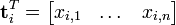
$\textbf{t}_i^T = \begin{bmatrix} x_{i,1} & \dots & x_{i,n} \end{bmatrix}$

Likewise, a column in this matrix will be a vector corresponding to a document, giving its relation to each term:

$\textbf{d}_j = \begin{bmatrix} x_{1,j} \\ \vdots \\ x_{m,j} \end{bmatrix}$

Now the dot product $\textbf{t}_i^T \textbf{t}_p$ between two term vectors gives the correlation between the terms over the documents. The matrix product $X X T$ contains all these dot products. Element $(i, p)$ (which is equal to element $(p, i)$ ) contains the dot product $\textbf{t}_i^T \textbf{t}_p$ ( $= \textbf{t}_p^T \textbf{t}_i$ ). 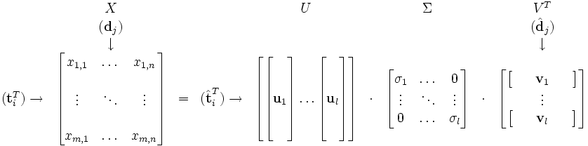Likewise, the matrix $X T X$ contains the dot products between all the document vectors, giving their correlation over the terms: $\textbf{d}_j^T \textbf{d}_q = \textbf{d}_q^T \textbf{d}_j$ .

Now assume that there exists a decomposition of $X$ such that $U$ and $V$ are orthonormal matrices and $Σ$ is a diagonal matrix. This is called a singular value decomposition (SVD):

X = U Σ V T

The matrix products giving us the term and document correlations then become

$\begin{matrix} X X^T &=& (U \Sigma V^T) (U \Sigma V^T)^T = (U \Sigma V^T) (V^{T^T} \Sigma^T U^T) = U \Sigma V^T V \Sigma^T U^T = U \Sigma \Sigma^T U^T \\ X^T X &=& (U \Sigma V^T)^T (U \Sigma V^T) = (V^{T^T} \Sigma^T U^T) (U \Sigma V^T) = V \Sigma U^T U \Sigma V^T = V \Sigma^T \Sigma V^T \end{matrix}$

Since $ΣΣ T$ and $Σ T Σ$ are diagonal we see that $U$ must contain the eigenvectors of $X X T$ , while $V$ must be the eigenvectors of $X T X$ . Both products have the same non-zero eigenvalues, given by the non-zero entries of $ΣΣ T$ , or equally, by the non-zero entries of $Σ T Σ$ . Now the decomposition looks like this:

$\begin{matrix} & X & & & U & & \Sigma & & V^T \\ & (\textbf{d}_j) & & & & & & & (\hat \textbf{d}_j) \\ & \downarrow & & & & & & & \downarrow \\ (\textbf{t}_i^T) \rightarrow & \begin{bmatrix} x_{1,1} & \dots & x_{1,n} \\ \\ \vdots & \ddots & \vdots \\ \\ x_{m,1} & \dots & x_{m,n} \\ \end{bmatrix} & = & (\hat \textbf{t}_i^T) \rightarrow & \begin{bmatrix} \begin{bmatrix} \, \\ \, \\ \textbf{u}_1 \\ \, \\ \,\end{bmatrix} \dots \begin{bmatrix} \, \\ \, \\ \textbf{u}_l \\ \, \\ \, \end{bmatrix} \end{bmatrix} & \cdot & \begin{bmatrix} \sigma_1 & \dots & 0 \\ \vdots & \ddots & \vdots \\ 0 & \dots & \sigma_l \\ \end{bmatrix} & \cdot & \begin{bmatrix} \begin{bmatrix} & & \textbf{v}_1 & & \end{bmatrix} \\ \vdots \\ \begin{bmatrix} & & \textbf{v}_l & & \end{bmatrix} \end{bmatrix} \end{matrix}$

The values $\sigma_1, \dots, \sigma_l$ are called the singular values, and $u_1, \dots, u_l$ and $v_1, \dots, v_l$ the left and right singular vectors. Notice how the only part of $U$ that contributes to $\textbf{t}_i$ is the $i'th$ row. Let this row vector be called $\hat \textrm{t}_i$ . Likewise, the only part of $V T$ that contributes to $\textbf{d}_j$ is the $j'th$ column, $\hat \textrm{d}_j$ . These are not the eigenvectors, but depend on all the eigenvectors.

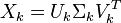
It turns out that when you select the $k$ largest singular values, and their corresponding singular vectors from $U$ and $V$ , you get the rank $k$ approximation to X with the smallest error (Frobenius norm). The amazing thing about this approximation is that not only does it have a minimal error, but it translates the term and document vectors into a concept space. The vector $\hat \textbf{t}_i$ then has $k$ entries, each giving the occurrence of term $i$ in one of the $k$ concepts. Likewise, the vector $\hat \textbf{d}_j$ gives the relation between document $j$ and each concept. We write this approximation as

$X_k = U_k \Sigma_k V_k^T$

You can now do the following:

See how related documents $j$ and $q$ are in the concept space by comparing the vectors $\hat \textbf{d}_j$ and $\hat \textbf{d}_q$ (typically by cosine similarity). This gives you a clustering of the documents.
Comparing terms $i$ and $p$ by comparing the vectors $\hat \textbf{t}_i$ and $\hat \textbf{t}_p$ , giving you a clustering of the terms in the concept space.
Given a query, view this as a mini document, and compare it to your documents in the concept space.

To do the latter, you must first translate your query into the concept space. It is then intuitive that you must use the same transformation that you use on your documents:

$\textbf{d}_j = U_k \Sigma_k \hat \textbf{d}_j$

$\hat \textbf{d}_j = \Sigma_k^{-1} U_k^T \textbf{d}_j$

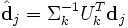
This means that if you have a query vector $q$ , you must do the translation $\hat \textbf{q} = \Sigma_k^{-1} U_k^T \textbf{q}$ before you compare it with the document vectors in the concept space. You can do the same for pseudo term vectors:

$\textbf{t}_i^T = \hat \textbf{t}_i^T \Sigma_k V_k^T$

$\hat \textbf{t}_i^T = \textbf{t}_i^T V_k^{-T} \Sigma_k^{-1} = \textbf{t}_i^T V_k \Sigma_k^{-1}$

$\hat \textbf{t}_i = \Sigma_k^{-1} V_k^T \textbf{t}_i$

[edit] Implementation

The SVD is typically computed using large matrix methods (for example, Lanczos methods) but may also be computed incrementally and with greatly reduced resources via a neural network-like approach, which does not require the large, full-rank matrix to be held in memory (Gorrell and Webb, 2005).

A fast, incremental, low-memory, large-matrix SVD algorithm has recently been developed (Brand, 2006). Unlike Gorrell and Webb's (2005) stochastic approximation, Brand's (2006) algorithm provides an exact solution.

[edit] Limitations

LSA has two drawbacks:

The resulting dimensions might be difficult to interpret. For instance, in

{(car), (truck), (flower)} --> {(1.3452 * car + 0.2828 * truck), (flower)}

the (1.3452 * car + 0.2828 * truck) component could be interpreted as "vehicle". However, it is very likely that cases close to

{(car), (bottle), (flower)} --> {(1.3452 * car + 0.2828 * bottle), (flower)}

will occur. This leads to results which can be justified on the mathematical level, but have no interpretable meaning in natural language.

The probabilistic model of LSA does not match observed data: LSA assumes that words and documents form a joint Gaussian model (ergodic hypothesis), while a Poisson distribution has been observed. Thus, a newer alternative is probabilistic latent semantic analysis, based on a multinomial model, which is reported to give better results than standard LSA^{[citation needed]}.

[edit] Commercial Applications

LSA has been used to assist in performing prior art searches for patents.^[1]

[edit] See also

An example of the application of [1] Latent Semantic Analysis in Natural language Processing
Compound term processing
Latent Dirichlet allocation
Latent semantic mapping
Latent Semantic Structure Indexing
Principal components analysis
Probabilistic latent semantic analysis
Spamdexing
Vectorial semantics

[edit] External links

Latent Semantic Analysis, a scholarpedia article on LSA written by Tom Landauer, one of the creators of LSA.
Latent Semantic Indexing, a non mathematical introduction and explanation of LSI
TheBirdsTheWord - Beta LSI Tool, A tool that emulates Google's semantic dictionary used to aide its ranking algorithm
The Semantic Indexing Project, an open source program for latent semantic indexing
SenseClusters, an open source package for Latent Semantic Analysis and other methods for clustering similar contexts

[edit] References

^ Gerry Elman, "Automated Patent Examination Support - A proposal", Biotechnology Law Report, October 2007

"The Latent Semantic Indexing home page". http://lsa.colorado.edu/.
Matthew Brand (2006). "Fast Low-Rank Modifications of the Thin Singular Value Decomposition". Linear Algebra and Its Applications 415: 20–30. doi:10.1016/j.laa.2005.07.021. http://www.merl.com/publications/TR2006-059/. -- a MATLAB implementation of Brand's algorithm is available
Thomas Landauer, P. W. Foltz, & D. Laham (1998). "Introduction to Latent Semantic Analysis" (PDF). Discourse Processes 25: 259–284. http://lsa.colorado.edu/papers/dp1.LSAintro.pdf.
S. Deerwester, Susan Dumais, G. W. Furnas, T. K. Landauer, R. Harshman (1990). "Indexing by Latent Semantic Analysis" (PDF). Journal of the American Society for Information Science 41 (6): 391–407. doi:10.1002/(SICI)1097-4571(199009)41:6<391::AID-ASI1>3.0.CO;2-9. http://lsi.research.telcordia.com/lsi/papers/JASIS90.pdf. Original article where the model was first exposed.
Michael Berry, S.T. Dumais, G.W. O'Brien (1995). Using Linear Algebra for Intelligent Information Retrieval. http://citeseer.ist.psu.edu/berry95using.html. PDF. Illustration of the application of LSA to document retrieval.
"Latent Semantic Analysis". InfoVis. http://iv.slis.indiana.edu/sw/lsa.html.
T. Hofmann (1999). "Probabilistic Latent Semantic Analysis" (PDF). Uncertainty in Artificial Intelligence.
G. Gorrell and B. Webb (2005). "Generalized Hebbian Algorithm for Latent Semantic Analysis" (PDF). Interspeech.
Fridolin Wild (November 23, 2005). "An Open Source LSA Package for R". CRAN. http://cran.at.r-project.org/web/packages/lsa/index.html. Retrieved on 2006-11-20.
Thomas Landauer. "A Solution to Plato's Problem: The Latent Semantic Analysis Theory of Acquisition, Induction, and Representation of Knowledge". http://www.welchco.com/02/14/01/60/96/02/2901.HTM. Retrieved on 2007-07-02.
Dimitrios Zeimpekis and E. Gallopoulos (September 11, 2005). "A MATLAB Toolbox for generating term-document matrices from text collections". http://scgroup.hpclab.ceid.upatras.gr/scgroup/Projects/TMG/. Retrieved on 2006-11-20.

[0] Gerry Elman, "Automated Patent Examination Support - A proposal", Biotechnology Law Report, October 2007

[1]

Latent semantic analysis

From Wikipedia, the free encyclopedia

Contents

[edit] Occurrence matrix

[edit] Applications

[edit] Rank lowering

[edit] Derivation

[edit] Implementation

[edit] Limitations

[edit] Commercial Applications

[edit] See also

[edit] External links

[edit] References

Views

Personal tools

Navigation

Search

Interaction

Toolbox

Languages