Bayes' theorem

From Wikipedia, the free encyclopedia

In probability theory, Bayes' theorem (often called Bayes' law after Rev Thomas Bayes) relates the conditional and marginal probabilities of two random events. It is often used to compute posterior probabilities given observations. For example, a patient may be observed to have certain symptoms. Bayes' theorem can be used to compute the probability that a proposed diagnosis is correct, given that observation. (See example 2)

As a formal theorem, Bayes' theorem is valid in all common interpretations of probability. However, it plays a central role in the debate around the foundations of statistics: frequentist and Bayesian interpretations disagree about the ways in which probabilities should be assigned in applications. Frequentists assign probabilities to random events according to their frequencies of occurrence or to subsets of populations as proportions of the whole, while Bayesians describe probabilities in terms of beliefs and degrees of uncertainty. The articles on Bayesian probability and frequentist probability discuss these debates in greater detail.

[edit] Statement of Bayes' theorem

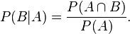
Bayes' theorem relates the conditional and marginal probabilities of events A and B, where B has a non-vanishing probability:

$P(A|B) = \frac{P(B | A)\, P(A)}{P(B)}.$

Each term in Bayes' theorem has a conventional name:

P(A) is the prior probability or marginal probability of A. It is "prior" in the sense that it does not take into account any information about B.
P(A|B) is the conditional probability of A, given B. It is also called the posterior probability because it is derived from or depends upon the specified value of B.
P(B|A) is the conditional probability of B given A.
P(B) is the prior or marginal probability of B, and acts as a normalizing constant.

Intuitively, Bayes' theorem in this form describes the way in which one's beliefs about observing 'A' are updated by having observed 'B'.

[edit] An example

Suppose there is a co-ed school having 60% boys and 40% girls as students. The girl students wear trousers or skirts in equal numbers; the boys all wear trousers. An observer sees a (random) student from a distance; all they can see is that this student is wearing trousers. What is the probability this student is a girl? The correct answer can be computed using Bayes' theorem.

The event A is that the student observed is a girl, and the event B is that the student observed is wearing trousers. To compute P(A|B), we first need to know:

P(A), or the probability that the student is a girl regardless of any other information. Since the observers sees a random student, meaning that all students have the same probability of being observed, and the fraction of girls among the students is 40%, this probability equals 0.4.
P(A'), or the probability that the student is a boy regardless of any other information (A' is the complementary event to A). This is 60%, or 0.6.
P(B|A), or the probability of the student wearing trousers given that the student is a girl. As they are as likely to wear skirts as trousers, this is 0.5.
P(B|A'), or the probability of the student wearing trousers given that the student is a boy. This is given as 1.
P(B), or the probability of a (randomly selected) student wearing trousers regardless of any other information. Since P(B) = P(B|A)P(A) + P(B|A')P(A'), this is 0.5×0.4 + 1×0.6 = 0.8.

Given all this information, the probability of the observer having spotted a girl given that the observed student is wearing trousers can be computed by substituting these values in the formula:

$P(A|B) = \frac{P(B|A) P(A)}{P(B)} = \frac{0.5 \times 0.4}{0.8} = 0.25.$

Another, essentially equivalent way of obtaining the same result is as follows. Assume, for concreteness, that there are 100 students, 60 boys and 40 girls. Among these, 60 boys and 20 girls wear trousers. All together there are 80 trouser-wearers, of which 20 are girls. Therefore the chance that a random trouser-wearer is a girl equals 20/80 = 0.25.

It is often helpful when calculating conditional probabilities to create a simple table containing the number of occurrences of each outcome, or the relative frequencies of each outcome, for each of the independent variables. The table below illustrates the use of this method for the above girl-or-boy example

	Girls	Boys	Total
Trousers	20	60	80
Skirts	20	0	20
Total	40	60	100

[edit] Derivation from conditional probabilities

To derive the theorem, we start from the definition of conditional probability. The probability of event A given event B is

$P(A|B)=\frac{P(A \cap B)}{P(B)}.$

Equivalently, the probability of event B given event A is

$P(B|A) = \frac{P(A \cap B)}{P(A)}. \!$

Rearranging and combining these two equations, we find

$P(A|B)\, P(B) = P(A \cap B) = P(B|A)\, P(A). \!$

This lemma is sometimes called the product rule for probabilities. Dividing both sides by P(B), provided that it is non-zero, we obtain Bayes' theorem:

$P(A|B) = \frac{P(A \cap B)}{P(B)} = \frac{P(B|A)\,P(A)}{P(B)}. \!$

[edit] Alternative forms of Bayes' theorem

Bayes' theorem is often completed by noting that, according to the Law of total probability,

$P(B) = P(A\cap B) + P(A^C\cap B) = P(B|A) P(A) + P(B|A^C) P(A^C).$

where A^C is the complementary event of A (often called "not A"). So the theorem can be restated as the following formula

$P(A|B) = \frac{P(B | A)\, P(A)}{P(B|A) P(A) + P(B|A^C) P(A^C)}. \!$

More generally, where {A_i} forms a partition of the event space,

$P(A_i|B) = \frac{P(B | A_i)\, P(A_i)}{\sum_j P(B|A_j)\,P(A_j)} , \!$

for any A_i in the partition.

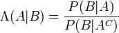
[edit] Bayes' theorem in terms of odds and likelihood ratio

Bayes' theorem can also be written neatly in terms of a likelihood ratio Λ and odds O as

$O(A|B)=O(A) \cdot \Lambda (A|B)$

where O(A|B) are the odds of A given B,

$O(A|B)=\frac{P(A|B)}{P(A^C|B)} \!$

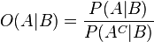
O(A) are the odds of A by itself

$O(A)=\frac{P(A)}{P(A^C)} \!$

and Λ(A|B) is the likelihood ratio.

$\Lambda (A|B) = \frac{P(B|A)}{P(B|A^C)} \!$

[edit] Bayes' theorem for probability densities

There is also a version of Bayes' theorem for continuous distributions. It is somewhat harder to derive, since probability densities are not probabilities, so Bayes' theorem has to be established by a limit process; see Papoulis (citation below), Section 7.3 for an elementary derivation.

Bayes originally used the proposition to find a continuous posterior distribution given discrete observations.

Bayes' theorem for probability densities is formally similar to the theorem for probabilities:

$f_X(x|Y=y) = \frac{f_{X,Y}(x,y)}{f_Y(y)} = \frac{f_Y(y|X=x)\,f_X(x)}{f_Y(y)} = \frac{f_Y(y|X=x)\,f_X(x)}{\int_{-\infty}^{\infty} f_Y(y|X=\xi )\,f_X(\xi )\,d\xi }.\!$

There is an analogous statement of the law of total probability, which is used in the denominator:

$f_Y(y) = \int_{-\infty}^{\infty} f_Y(y|X=x )\,f_X(x)\,dx .\!$

As in the discrete case, the terms have standard names.

$f_{X,Y}(x,y)\,$

is the joint density function of X and Y,

$f_X(x|Y=y)\,$

is the posterior probability density function of X given Y = y,

$f_Y(y|X=x) = L(x|y)\,$

is (as a function of x) the likelihood function of X given Y = y, and

$f_X(x)\,$

and

$f_Y(y)\!$

are the marginal probability density functions of X and Y respectively, where ƒ_X(x) is the prior probability density function of X.

[edit] Abstract Bayes' theorem

Given two absolutely continuous probability measures $P ˜ Q$ on the probability space $(\Omega, \mathcal{F})$ and a sigma-algebra $\mathcal{G} \subset \mathcal{F}$ , the abstract Bayes theorem for a $\mathcal{F}$ -measurable random variable $X$ becomes

$E_P \left[ X|\mathcal{G} \right] = \frac{E_Q \left[ \left.\frac{dP}{dQ} X \right|\mathcal{G} \right] }{E_Q \left[ \frac{dP}{dQ}|\mathcal{G} \right] } .$

Proof :

by definition of conditional probability,

$E_P \left[ X|\mathcal{G} \right] = \frac{E_P \left[ X 1_\mathcal{G} \right] }{P \left[ \mathcal{G} \right] } = \frac{E_P \left[ X 1_\mathcal{G} \right] }{E_P \left[ 1_\mathcal{G} \right] }$

We further have that

$E_Q \left[ \frac{dP}{dQ} X\right] = \int \frac{dP}{dQ} X \,dQ = \int X \, dP = E_P \left[ X \right].$

Hence,

$E_Q \left[ \left.\frac{dP}{dQ} X\right|\mathcal{G} \right] = \frac{E_Q \left[ \frac{dP}{dQ} X 1_\mathcal{G} \right] }{E_Q \left[ 1_\mathcal{G} \right] } = \frac{E_P \left[ X 1_\mathcal{G} \right] }{E_Q \left[ 1_\mathcal{G} \right] }$

$E_Q \left[ \left.\frac{dP}{dQ}\right|\mathcal{G} \right] = \frac{E_Q \left[ \frac{dP}{dQ} 1_\mathcal{G} \right] }{E_Q \left[ 1_\mathcal{G} \right] } = \frac{E_P \left[ 1_\mathcal{G} \right] }{E_Q \left[ 1_\mathcal{G} \right] }.$

Summarizing, we obtain the desired result.

This formulation is used in Kalman filtering to find Zakai equations. It is also used in financial mathematics for change of numeraire techniques.

[edit] Extensions of Bayes' theorem

Theorems analogous to Bayes' theorem hold in problems with more than two variables. For example:

$P(A|B \cap C) = \frac{P(A) \, P(B|A) \, P(C|A \cap B)}{P(B) \, P(C|B)}\,.$

This can be derived in a few steps from Bayes' theorem and the definition of conditional probability:

$P(A|B \cap C) = \frac{P(A \cap B \cap C)}{P(B \cap C)} = \frac{P(C|A \cap B) \, P(A \cap B)}{P(B) \, P(C|B)} = \frac{P(A) \, P(B|A) \, P(C|A \cap B)}{P(B) \, P(C|B)}\,.$

Similarly,

$P(A|B \cap C) = \frac{P(B|A \cap C) \, P(A|C)}{P(B|C)}\,,$

which can be regarded as a conditional Bayes' Theorem, and can be derived by as follows:

$P(A|B \cap C) = \frac{P(A \cap B \cap C)}{P(B \cap C)} = \frac{P(B|A \cap C) \, P(A|C) \, P(C)}{P(C) \, P(B|C)} = \frac{P(B|A \cap C) \, P(A|C)}{P(B|C)}\,.$

A general strategy is to work with a decomposition of the joint probability, and to marginalize (integrate) over the variables that are not of interest. Depending on the form of the decomposition, it may be possible to prove that some integrals must be 1, and thus they fall out of the decomposition; exploiting this property can reduce the computations very substantially. A Bayesian network, for example, specifies a factorization of a joint distribution of several variables in which the conditional probability of any one variable given the remaining ones takes a particularly simple form (see Markov blanket).

[edit] Further examples

[edit] Example 1: Drug testing

Bayes' theorem is useful in evaluating the result of drug tests. Suppose a certain drug test is 99% sensitive and 99% specific, that is, the test will correctly identify a drug user as testing positive 99% of the time, and will correctly identify a non-user as testing negative 99% of the time. This would seem to be a relatively accurate test, but Bayes' theorem will reveal a potential flaw. Let's assume a corporation decides to test its employees for opium use, and 0.5% of the employees use the drug. We want to know the probability that, given a positive drug test, an employee is actually a drug user. Let "D" be the event of being a drug user and "N" indicate being a non-user. Let "+" be the event of a positive drug test. We need to know the following:

P(D), or the probability that the employee is a drug user, regardless of any other information. This is 0.005, since 0.5% of the employees are drug users. This is the prior probability of D.
P(N), or the probability that the employee is not a drug user. This is 1 − P(D), or 0.995.
P(+|D), or the probability that the test is positive, given that the employee is a drug user. This is 0.99, since the test is 99% accurate.
P(+|N), or the probability that the test is positive, given that the employee is not a drug user. This is 0.01, since the test will produce a false positive for 1% of non-users.
P(+), or the probability of a positive test event, regardless of other information. This is 0.0149 or 1.49%, which is found by adding the probability that a true positive result will appear (= 99% x 0.5% = 0.495%) plus the probability that a false positive will appear (= 1% x 99.5% = 0.995%). This is the prior probability of +.

Given this information, we can compute the posterior probability P(D|+) of an employee who tested positive actually being a drug user:

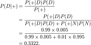
$\begin{align}P(D|+) & = \frac{P(+ | D) P(D)}{P(+)} \\ & = \frac{P(+ | D) P(D)}{P(+ | D) P(D) + P(+ | N) P(N)} \\ & = \frac{0.99 \times 0.005}{0.99 \times 0.005 + 0.01 \times 0.995} \\ & = 0.3322.\end{align}$

Despite the apparently high accuracy of the test, the probability that an employee who tested positive actually did use drugs is only about 33%, so it is actually more likely that the employee is not a drug user. The rarer the condition for which we are testing, the greater the percentage of positive tests that will be false positives.

[edit] Example 2: Bayesian inference

Applications of Bayes' theorem often assume the philosophy underlying Bayesian probability that uncertainty and degrees of belief can be measured as probabilities. One such example follows. For additional worked out examples, including simpler examples, please see the article on the examples of Bayesian inference.

We describe the marginal probability distribution of a variable A as the prior probability distribution or simply the 'prior'. The conditional distribution of A given the "data" B is the posterior probability distribution or just the 'posterior'.

Suppose we wish to know about the proportion r of voters in a large population who will vote "yes" in a referendum. Let n be the number of voters in a random sample (chosen with replacement, so that we have statistical independence) and let m be the number of voters in that random sample who will vote "yes". Suppose that we observe n = 10 voters and m = 7 say they will vote yes. From Bayes' theorem we can calculate the probability distribution function for r using

$f(r | n=10, m=7) = \frac {f(m=7 | r, n=10) \, f(r)} {\int_0^1 f(m=7|r, n=10) \, f(r) \, dr}. \!$

From this we see that from the prior probability density function f(r) and the likelihood function L(r) = f(m = 7|r, n = 10), we can compute the posterior probability density function f(r|n = 10, m = 7).

The prior probability density function f(r) summarizes what we know about the distribution of r in the absence of any observation. We provisionally assume in this case that the prior distribution of r is uniform over the interval [0, 1]. That is, f(r) = 1. If some additional background information is found, we should modify the prior accordingly. However before we have any observations, all outcomes are equally likely.

Under the assumption of random sampling, choosing voters is just like choosing balls from an urn. The likelihood function L(r) = P(m = 7|r, n = 10,) for such a problem is just the probability of 7 successes in 10 trials for a binomial distribution.

$P( m=7 | r, n=10) = {10 \choose 7} \, r^7 \, (1-r)^3.$

As with the prior, the likelihood is open to revision -- more complex assumptions will yield more complex likelihood functions. Maintaining the current assumptions, we compute the normalizing factor,

$\begin{align} \int_0^1 P( m=7|r, n=10) \, f(r) \, dr & = \int_0^1 {10 \choose 7} \, r^7 \, (1-r)^3 \, 1 \, dr \\ & = {10 \choose 7} \left / {11 \choose 3,7,1} \right . = {10 \choose 7} \, \frac{1}{1320} \end{align}$

and the posterior distribution for r is then

$f(r | n=10, m=7) = \frac{{10 \choose 7} \, r^7 \, (1-r)^3 \, 1} {{10 \choose 7} \, \frac{1}{1320}} = 1320 \, r^7 \, (1-r)^3$

for r between 0 and 1, inclusive.

One may be interested in the probability that more than half the voters will vote "yes". The prior probability that more than half the voters will vote "yes" is 1/2, by the symmetry of the uniform distribution. In comparison, the posterior probability that more than half the voters will vote "yes", i.e., the conditional probability given the outcome of the opinion poll – that seven of the 10 voters questioned will vote "yes" – is

$1320\int_{1/2}^1 r^7(1-r)^3\,dr \approx 0.887, \!$

which is about an "89% chance".

[edit] Example 3: The Monty Hall problem

Main article: Monty Hall problem

We are presented with three doors to choose - red, green, and blue - one of which has a prize hidden behind it. We choose the red door. The presenter, who knows where the prize is, opens the blue door and reveals that there is no prize behind it. He then asks if we wish to change our mind about our initial selection of red. Will changing our mind at this point improve our chances of winning the prize?

You might think that, with two doors left unopened, you have a 50:50 chance with either door, and so there is no point in changing doors. However, this is not the case. Let us call the situation that the prize is behind a given door A_r, A_g, and A_b.

To start with, $P(A_r) = P(A_g) = P(A_b) = \frac 1 3$ , and to make things simpler we shall assume that we have already picked the red door.

Let us call B "the presenter opens the blue door". Without any prior knowledge, we would assign this a probability of 50%.

In the situation where the prize is behind the red door, the presenter is free to pick between the green or the blue door at random. Thus, $P (B | A r) = 1 / 2$
In the situation where the prize is behind the green door, the presenter must pick the blue door. Thus, $P (B | A g) = 1$
In the situation where the prize is behind the blue door, the presenter must pick the green door. Thus, $P (B | A b) = 0$

Thus,

$\begin{align} P(A_r|B) & = \frac{P(B | A_r) P(A_r)}{P(B)} = \frac{\frac 1 2 \cdot \frac 1 3}{\frac 1 2} = \frac 1 3 \\ P(A_g|B) & = \frac{P(B | A_g) P(A_g)}{P(B)} = \frac{1 \cdot \frac 1 3}{\frac 1 2} = \frac 2 3 \\ P(A_b|B) & = \frac{P(B | A_b) P(A_b)}{P(B)} = \frac{0 \cdot \frac 1 3}{\frac 1 2} = 0. \end{align}$

So, we should always choose the green door.

Note how this depends on the value of P(B). Another way of looking at the apparent inconsistency is that, when you chose the first door, you had a 1/3 chance of being right. When the second door was removed from the list of possibilities, this left the last door with a 2/3 chance of being right.

[edit] Historical remarks

An investigation by a statistics professor (Stigler 1983) suggests that Bayes' theorem was discovered by Nicholas Saunderson some time before Bayes. However, this interpretation is argued against in (Edwards 1986).

Bayes' theorem is named after the Reverend Thomas Bayes (1702–1761), who studied how to compute a distribution for the parameter of a binomial distribution (to use modern terminology). His friend, Richard Price, edited and presented the work in 1763, after Bayes' death, as An Essay towards solving a Problem in the Doctrine of Chances. Pierre-Simon Laplace replicated and extended these results in an essay of 1774, apparently unaware of Bayes' work.

One of Bayes' results (Proposition 5) gives a simple description of conditional probability, and shows that it can be expressed independently of the order in which things occur:

If there be two subsequent events, the probability of the second b/N and the probability of both together P/N, and it being first discovered that the second event has also happened, from hence I guess that the first event has also happened, the probability I am right [i.e., the conditional probability of the first event being true given that the second has also happened] is P/b.

Note that the expression says nothing about the order in which the events occurred; it measures correlation, not causation. His preliminary results, in particular Propositions 3, 4, and 5, imply the result now called Bayes' Theorem (as described above), but it does not appear that Bayes himself emphasized or focused on that result

Bayes' main result (Proposition 9 in the essay) is the following: assuming a uniform distribution for the prior distribution of the binomial parameter p, the probability that p is between two values a and b is

$\frac {\int_a^b {n+m \choose m} p^m (1-p)^n\,dp} {\int_0^1 {n+m \choose m} p^m (1-p)^n\,dp} \!$

where m is the number of observed successes and n the number of observed failures.

What is "Bayesian" about Proposition 9 is that Bayes presented it as a probability for the parameter p. So, one can compute probability for an experimental outcome, but also for the parameter which governs it, and the same algebra is used to make inferences of either kind.

Bayes states his question in a way that might make the idea of assigning a probability distribution to a parameter palatable to a frequentist. He supposes that a billiard ball is thrown at random onto a billiard table, and that the probabilities p and q are the probabilities that subsequent billiard balls will fall above or below the first ball.

Stephen Fienberg [1] describes the evolution of the field from "inverse probability" at the time of Bayes and Laplace, and even of Harold Jeffreys (1939) to "Bayesian" in the 1950's. The irony is that this label was introduced by R.A. Fisher in a derogatory sense. So, historically, Bayes was not a "Bayesian". It is actually unclear whether or not he was a Bayesian in the modern sense of the term, i.e. whether or not he was interested in inference or merely in probability: the 1763 essay is more of a probability paper.

[edit] See also

[edit] References

[edit] Versions of the essay

Thomas Bayes (1763), "An Essay towards solving a Problem in the Doctrine of Chances. By the late Rev. Mr. Bayes, F. R. S. communicated by Mr. Price, in a letter to John Canton, A. M. F. R. S.", Philosophical Transactions, Giving Some Account of the Present Undertakings, Studies and Labours of the Ingenious in Many Considerable Parts of the World 53:370–418.
Thomas Bayes (1763/1958) "Studies in the History of Probability and Statistics: IX. Thomas Bayes' Essay Towards Solving a Problem in the Doctrine of Chances", Biometrika 45:296–315. (Bayes' essay in modernized notation)
Thomas Bayes "An essay towards solving a Problem in the Doctrine of Chances". (Bayes' essay in the original notation)

[edit] Commentaries

G. A. Barnard (1958) "Studies in the History of Probability and Statistics: IX. Thomas Bayes' Essay Towards Solving a Problem in the Doctrine of Chances", Biometrika 45:293–295. (biographical remarks)
Daniel Covarrubias. "An Essay Towards Solving a Problem in the Doctrine of Chances". (an outline and exposition of Bayes' essay)
Stephen M. Stigler (1982). "Thomas Bayes' Bayesian Inference," Journal of the Royal Statistical Society, Series A, 145:250–258. (Stigler argues for a revised interpretation of the essay; recommended)
Isaac Todhunter (1865). A History of the Mathematical Theory of Probability from the time of Pascal to that of Laplace, Macmillan. Reprinted 1949, 1956 by Chelsea and 2001 by Thoemmes.
An Intuitive Explanation of Bayesian Reasoning (includes biography)

[edit] Additional material

Pierre-Simon Laplace (1774/1986), "Memoir on the Probability of the Causes of Events", Statistical Science 1(3):364–378.
Stephen M. Stigler (1986), "Laplace's 1774 memoir on inverse probability", Statistical Science 1(3):359–378.
Stephen M. Stigler (1983), "Who Discovered Bayes' Theorem?" The American Statistician 37(4):290–296.
A. W. F. Edwards (1986), "Is the Reference in Hartley (1749) to Bayesian Inference?", The American Statistician 40(2):109–110.
Jeff Miller, et al., Earliest Known Uses of Some of the Words of Mathematics (B). (very informative; recommended)
Athanasios Papoulis (1984), Probability, Random Variables, and Stochastic Processes, second edition. New York: McGraw-Hill.
The on-line textbook: Information Theory, Inference, and Learning Algorithms, by David J. C. MacKay provides an up to date overview of the use of Bayes' theorem in information theory and machine learning.
Bayes' Theorem entry in the Stanford Encyclopedia of Philosophy by James Joyce, provides a comprehensive introduction to Bayes' theorem.
Stanford Encyclopedia of Philosophy: Inductive Logic provides a comprehensive Bayesian treatment of Inductive Logic and Confirmation Theory.
Eric W. Weisstein, Bayes' Theorem at MathWorld.
Bayes' theorem at PlanetMath.
Eliezer S. Yudkowsky (2003), "An Intuitive Explanation of Bayesian Reasoning"
A tutorial on probability and Bayes’ theorem devised for Oxford University psychology students
Confirmation Theory An extensive presentation of Bayesian Confirmation Theory