Ackermann function

From Wikipedia, the free encyclopedia

In computability theory, the Ackermann function or Ackermann–Péter function is a simple example of a computable function that is not primitive recursive. The set of primitive recursive functions is a subset of the set of general recursive functions. Ackermann's function is an example that shows that the former is a strict subset of the latter.

The Ackermann function is defined recursively for non-negative integers m and n as follows:

$A(m, n) = \begin{cases} n+1 & \mbox{if } m = 0 \\ A(m-1, 1) & \mbox{if } m > 0 \mbox{ and } n = 0 \\ A(m-1, A(m, n-1)) & \mbox{if } m > 0 \mbox{ and } n > 0. \end{cases}$

Its value grows rapidly, even for small inputs. For example A(4,2) contains 19,729 decimal digits.^[1]

[edit] History

In the late 1920s, the mathematicians Gabriel Sudan and Wilhelm Ackermann, students of David Hilbert, were studying the foundations of computation. Sudan is credited with inventing the lesser-known Sudan function, the first published function that is recursive but not primitive recursive. Shortly afterwards and independently, in 1928, Ackermann published his own recursive but not primitive recursive function.^[2]

Ackermann originally considered a function A(m, n, p) of three variables, the p-fold iterated exponentiation of m with n, or m → n → p as expressed using the Conway chained arrow notation. When p = 1, this is mⁿ, which is m multiplied by itself n times. When p = 2, it is a tower of exponents ${{m^m}^{{\cdot}^{{\cdot}^{{\cdot}^m}}}}$ with n levels, or m raised n times to the power m also written as ⁿm, the tetration of m with n. This can be generalized indefinitely as p becomes larger.

Ackermann proved that A is a recursive function, a function that a computer with unbounded memory can calculate, but it is not a primitive recursive function, a class of functions including almost all familiar functions such as addition and factorial.

In On the Infinite, David Hilbert hypothesized that the Ackermann function was not primitively recursive, but it was Ackermann, Hilbert’s personal secretary and former student, who actually proved the hypothesis in his paper On Hilbert’s Construction of the Real Numbers. On the Infinite was Hilbert’s most important paper on the foundations of mathematics, serving as the heart of Hilbert's program to secure the foundation of transfinite numbers by basing them on finite methods.^[3]^[4]

A similar function of only two variables was later defined by Rózsa Péter and Raphael Robinson; its definition is given below. The numbers, except in the first few rows, are three less than powers of two. For the exact relation between the two functions, see below.^[5]

[edit] Definition and properties

The Ackermann function is defined recursively for non-negative integers m and n as follows (this presentation is due to Rózsa Péter):

$A(m, n) = \begin{cases} n+1 & \mbox{if } m = 0 \\ A(m-1, 1) & \mbox{if } m > 0 \mbox{ and } n = 0 \\ A(m-1, A(m, n-1)) & \mbox{if } m > 0 \mbox{ and } n > 0. \end{cases}$

It may not be immediately obvious that the evaluation of these functions always terminates. The recursion is bounded because in each recursive application either m decreases, or m remains the same and n decreases. Each time that n reaches zero, m decreases, so m eventually reaches zero as well. (Expressed more technically, in each case the pair (m, n) decreases in the lexicographic order, which preserves the well-ordering of the non-negative integers.) However, when m decreases there is no upper bound on how much n can increase — and it will often increase greatly.

The Ackermann function can also be expressed nonrecursively using:

Conway chained arrow notation:

A(m, n) = (2 → (n+3) → (m − 2)) − 3 for m > 2

hence

2 → n → m = A(m+2,n-3) + 3 for n>2.

(n=1 and n=2 would correspond with A(m,−2) = −1 and A(m,−1) = 1, which could logically be added.)

hyper operators:

A(m, n) = hyper(2, m, n + 3) − 3.

the indexed version of Knuth's up-arrow notation:

A(m, n) = $2\uparrow^{m-2} (n+3) - 3.$

The part of the definition A(m, 0) = A(m-1, 1) corresponds to $2\uparrow^{m+1} 3=2\uparrow^m 4.$

For small values of m like 1, 2, or 3, the Ackermann function grows relatively slowly with respect to n (at most exponentially). For m ≥ 4, however, it grows much more quickly; even A(4, 2) is about 2×10¹⁹⁷²⁸, and the decimal expansion of A(4, 3) is very large by any typical measure.

If we define the function f (n) = A(n, n), which increases both m and n at the same time, we have a function of one variable that dwarfs every primitive recursive function, including very fast-growing functions such as the exponential function, the factorial function, multi- and superfactorial functions, and even functions defined using Knuth's up-arrow notation (except when the indexed up-arrow is used).

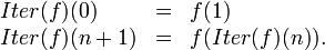
This extreme growth can be exploited to show that f, which is obviously computable on a machine with infinite memory such as a Turing machine and so is a computable function, grows faster than any primitive recursive function and is therefore not primitive recursive. Though the Ackermann function is often used to debunk the hypothesis that all useful or simple functions are primitive recursive, one should not confuse the primitive recursive functions with those definable by primitive recursion (it is this latter class that is of interest to programming language theorists because programs written using only primitive recursion are guaranteed to terminate). In a category with exponentials, using the isomorphism $A \times B \rightarrow C \cong A \rightarrow (B \rightarrow C)$ , the Ackermann function may be defined via primitive recursion over higher-order functionals as follows:

$\begin{array}{lcl} Ack(0) & = & Succ \\ Ack(m+1) & = & Iter(Ack(m)) \end{array}$

where Succ is the usual successor function and Iter is defined by primitive recursion as well:

$\begin{array}{lcl} Iter(f)(0) & = & f(1) \\ Iter(f)(n+1) & = & f(Iter(f)(n)). \end{array}$

One interesting aspect of the Ackermann function is that the only arithmetic operations it ever uses are addition and subtraction of 1. Its properties come solely from the power of unlimited recursion. This also implies that its running time is at least proportional to its output, and so is also extremely huge. In actuality, for most cases the running time is far larger than the output; see below.

[edit] Table of values

Computing the Ackermann function can be restated in terms of an infinite table. We place the natural numbers along the top row. To determine a number in the table, take the number immediately to the left, then look up the required number in the previous row, at the position given by the number just taken. If there is no number to its left, simply look at column 1 in the previous row. Here is a small upper-left portion of the table:

Values of A(m, n)
m\n	0	1	2	3	4	n
0	1	2	3	4	5	$n + 1$
1	2	3	4	5	6	$n + 2 = 2 + (n + 3) - 3$
2	3	5	7	9	11	$2n + 3 = 2\cdot(n + 3) - 3$
3	5	13	29	61	125	$2 (n + 3) - 3$
4	13	65533	2⁶⁵⁵³⁶ − 3	${2^{2^{65536}}} - 3$	A(3, A(4, 3))	$\begin{matrix}\underbrace{{2^2}^{{\cdot}^{{\cdot}^{{\cdot}^2}}}} - 3 \\n\mbox{ + 3 twos}\end{matrix}$
5	65533	$\begin{matrix}\underbrace{{2^2}^{{\cdot}^{{\cdot}^{{\cdot}^2}}}} - 3 \\65536\mbox{ twos}\end{matrix}$	A(4, A(5, 1))	A(4, A(5, 2))	A(4, A(5, 3))	A(4, A(5, n-1))
6	A(5, 1)	A(5, A(6, 0))	A(5, A(6, 1))	A(5, A(6, 2))	A(5, A(6, 3))	A(5, A(6, n-1))

The numbers listed here in a recursive reference are very large and cannot be easily notated in some other form.

Despite the large values occurring in this early section of the table, some even larger numbers have been defined, such as Graham's number, which cannot be written with any small number of Knuth arrows. This number is constructed with a technique similar to applying the Ackermann function to itself recursively.

This is a repeat of the above table, but with the values replaced by the relevant expression from the function definition to show the pattern clearly:

Values of A(m, n)
m\n	0	1	2	3	4	n
0	0+1	1+1	2+1	3+1	4+1	$n + 1$
1	A(0,1)	A(0,A(1,0))	A(0,A(1,1))	A(0,A(1,2))	A(0,A(1,3))	$n + 2 = 2 + (n + 3) - 3$
2	A(1,1)	A(1,A(2,0))	A(1,A(2,1))	A(1,A(2,2))	A(1,A(2,3))	$2n + 3 = 2\cdot(n + 3) - 3$
3	A(2,1)	A(2,A(3,0))	A(2,A(3,1))	A(2,A(3,2))	A(2,A(3,3))	$2 (n + 3) - 3$
4	A(3,1)	A(3,A(4,0))	A(3,A(4,1))	A(3,A(4,2))	A(3,A(4,3))	$\begin{matrix}\underbrace{{2^2}^{{\cdot}^{{\cdot}^{{\cdot}^2}}}} - 3 \\n\mbox{ + 3 twos}\end{matrix}$
5	A(4,1)	A(4,A(5,0))	A(4,A(5,1))	A(4,A(5,2))	A(4,A(5,3))	A(4, A(5, n-1))
6	A(5,1)	A(5,A(6,0))	A(5,A(6,1))	A(5,A(6,2))	A(5,A(6,3))	A(5, A(6, n-1))

[edit] Extension

f=A(4,z) in the complex z-plane. Levels, corresponding to integer values of the Re(f) and those for Im(f) are drawn^[6]

The first three of Ackermann functions can be expressed through elementary functions; they allow straightforward analytic extension for complex values of the second argument. In these sense, A(1,z), A(2,z), A(3,z) are analytic functions in the whole z-plane.

No such extension is yet established for A(m,z) at integer m>3. The sketch in the figure at right represents the possible realization of such extension, that remains limited at $\pm i \infty$ . The drawing indicates that, perhaps, the extension of A(4,z), analytic in the whole z-plane, is not possible; the analytic extension should have singularity at z=-5 and cut at the real axis for z<-5. Such cut and singularities seem to be typical also for the tetration function.

[edit] Expansion

To see how the Ackermann function grows so quickly, it helps to expand out some simple expressions using the rules in the original definition. For example, we can fully evaluate $A (1,2)$ in the following way:

$\begin{align} A(1,2) & = A(0, A(1, 1)) \\ & = A(0, A(0, A(1, 0))) \\ & = A(0, A(0, A(0, 1))) \\ & = A(0, A(0, 2)) \\ & = A(0, 3) \\ & = 4. \end{align}$

To demonstrate how $A (4,3)$ 's computation results in many steps and in a large number:

$\begin{align} A(4, 3) & = A(3, A(4, 2)) \\ & = A(3, A(3, A(4, 1))) \\ & = A(3, A(3, A(3, A(4, 0)))) \\ & = A(3, A(3, A(3, A(3, 1)))) \\ & = A(3, A(3, A(3, A(2, A(3, 0))))) \\ & = A(3, A(3, A(3, A(2, A(2, 1))))) \\ & = A(3, A(3, A(3, A(2, A(1, A(2, 0)))))) \\ & = A(3, A(3, A(3, A(2, A(1, A(1, 1)))))) \\ & = A(3, A(3, A(3, A(2, A(1, A(0, A(1, 0))))))) \\ & = A(3, A(3, A(3, A(2, A(1, A(0, A(0, 1))))))) \\ & = A(3, A(3, A(3, A(2, A(1, A(0, 2)))))) \\ & = A(3, A(3, A(3, A(2, A(1, 3))))) \\ & = A(3, A(3, A(3, A(2, A(0, A(1, 2)))))) \\ & = A(3, A(3, A(3, A(2, A(0, A(0, A(1, 1))))))) \\ & = A(3, A(3, A(3, A(2, A(0, A(0, A(0, A(1, 0)))))))) \\ & = A(3, A(3, A(3, A(2, A(0, A(0, A(0, A(0, 1)))))))) \\ & = A(3, A(3, A(3, A(2, A(0, A(0, A(0, 2)))))) \\ & = A(3, A(3, A(3, A(2, A(0, A(0, 3))))) \\ & = A(3, A(3, A(3, A(2, A(0, 4))))) \\ & = A(3, A(3, A(3, A(2, 5)))) \\ & = ... \\ & = A(3, A(3, A(3, 13))) \\ & = ... \\ & = A(3, A(3, 65533)) \\ & = ... \\ & = A(3, 2^{65536} - 3) \\ & = ... \\ & = 2^{2^{ \overset{65536}{} }} - 3. \\ \end{align}$

Written as a power of 10, this is roughly equivalent to 10^{10^19727.78}.

[edit] Inverse

Since the function f (n) = A(n, n) considered above grows very rapidly, its inverse function, f⁻¹, grows very slowly. This inverse Ackermann function f⁻¹ is usually denoted by α. In fact, α(n) is less than 5 for any conceivable input size n, since A(4, 4) is on the order of $2^{2^{10^{19729}}}$ .

This inverse appears in the time complexity of some algorithms, such as the disjoint-set data structure and Chazelle's algorithm for minimum spanning trees. Sometimes Ackermann's original function or other variations are used in these settings, but they all grow at similarly high rates. In particular, some modified functions simplify the expression by eliminating the −3 and similar terms.

A two-parameter variation of the inverse Ackermann function can be defined as follows:

$\alpha(m,n) = \min\{i \geq 1 : A(i,\lfloor m/n \rfloor) \geq \log_2 n\}.$

This function arises in more precise analyses of the algorithms mentioned above, and gives a more refined time bound. In the disjoint-set data structure, m represents the number of operations while n represents the number of elements; in the minimum spanning tree algorithm, m represents the number of edges while n represents the number of vertices. Several slightly different definitions of α(m, n) exist; for example, log₂ n is sometimes replaced by n, and the floor function is sometimes replaced by a ceiling.

Other studies might define an inverse function of one where m is set to a constant, such that the inverse applies to a particular row.^[7]

[edit] Use as benchmark

The Ackermann function, due to its definition in terms of extremely deep recursion, can be used as a benchmark of a compiler's ability to optimize recursion. The first use of Ackermann's function in this way was by Yngve Sundblad, The Ackermann function. A Theoretical, computational and formula manipulative study. (BIT 11 (1971), 107119).

This seminal paper was taken up by Brian Wichmann (co-author of the Whetstone benchmark) in a trilogy of papers written between 1975 and 1982.^[8]^[9]^[10]

A more recent use of Ackermann's function as a compiler benchmark is in The Computer Language Shootout which compares the time required to evaluate this function for fixed arguments in many different programming language implementations.^[11]^[12]

For example, a compiler which, in analyzing the computation of A(3, 30), is able to save intermediate values like the A(3, n) and A(2, n) in that calculation rather than recomputing them, can speed up computation of A(3, 30) by a factor of hundreds of thousands. Also, if A(2, n) is computed directly rather than as a recursive expansion of the form A(1, A(1, A(1,...A(1, 0)...))), this will save significant amounts of time. Computing A(1, n) takes linear time in n. Computing A(2, n) requires quadratic time, since it expands to O(n) nested calls to A(1, i) for various i. Computing A(3, n) requires time proportionate to 4ⁿ⁺¹. The computation of A(3, 1) in the example above takes 16 (4²) steps.

A(4, 2), which appears as a decimal expansion in several web pages, cannot possibly be computed by simple recursive application of the Ackermann function in any tractable amount of time. Instead, shortcut formulas such as A(3, n) = 8×2ⁿ−3 are used as an optimization to complete some of the recursive calls.

A practical method of computing functions similar to Ackermann's is to use memoization of intermediate results. A compiler could apply this technique to a function automatically using Donald Michie's "memo functions".^[13]^{[citation needed]}

[edit] Ackermann numbers

Related to the Ackermann function but in fact different are the Ackermann numbers, a sequence where the n^th term equals:

$\begin{matrix} n\ \underbrace{\uparrow\dots\uparrow}\ n \\ n \end{matrix}$

in the Knuth's up-arrow notation, or

$n \to n \to n$

in the Conway chained arrow notation.^[14]

For instance, the first three Ackermann numbers are

1 $\uparrow$ 1,
2 $\uparrow\uparrow$ 2
3 $\uparrow\uparrow\uparrow$ 3

which equal the following:

1¹ = 1
${\ ^{2}2}$ = 4
${\ ^{^{^3}3}3} = 3\uparrow\uparrow3\uparrow\uparrow3 = \begin{matrix} \underbrace{\qquad\quad3^{3^{3^{3^{3^{3^{.^{.^{.^{3}}}}}}}}}\qquad\quad} \\ 3^{27}{\rm\ or\ } 7625597484987{\rm\ threes}\end{matrix}$

An attempt to express the fourth Ackermann number, 4 $\uparrow\uparrow\uparrow\uparrow$ 4, using iterated exponentiation as above would become extremely complicated. However, it can be expressed using tetration in three nested layers as shown below. Explanation: in the middle layer, there is a tower of tetration whose full length is $^{^{^{^4}4}4}4$ and the final result is the top layer of tetrated 4's whose full length equals the calculation of the middle layer. Note that by way of size comparison, the simple expression $^{^4}4$ already exceeds a googolplex, so the fourth Ackermann number is quite large.

$\begin{matrix} \underbrace{\begin{matrix} \underbrace{^{^{^{^{^{^{^{4}.}.}.}4}4}4}4} \\ ^{^{^{^{^{^{^{4}.}.}.}4}4}4}4 \end{matrix}} \\ ^{^{^{^4}4}4}4 \end{matrix}$

[edit] In popular culture

Randall Munroe has mentioned the Ackermann function in his popular web-comic xkcd.^[15] In the comic, Munroe makes reference to the Ackermann function with Graham's number as the arguments. He named it "The xkcd number".^[16]

However, it should be noted that although it might seem like a big step up from Graham's Number, the xkcd number is not even as big as $g 65$ (with $g 64$ being Graham's number), considering the recursive definition of:

$g_0=4,\ g_n = 3\uparrow^{g_{n-1}}3$

Proof:

$xkcd number = A(G,G) = 2\uparrow^{G-2}G-3$

$g_{65}=3\uparrow^{G}3$

$3\uparrow^{G}3>>3\uparrow^{G-1}G>>2\uparrow^{G-2}G-3 = A(G,G)$

This shows how functions and methods that produce huge number such as the Moser number or Graham's Number grow so quickly, that not even concepts like the xkcd number cause any significant growth. Not even $g G$ , ${g_g}_G$ , ${{g_g}_g}_G$ or any such a tower would be significant given the possibilities of the Conway chained arrow notation, per example.

A question involving this function was posed at the International Mathematical Olympiad, the most significant mathematics competition for school age students, in 1981.^[17]

[edit] See also

[edit] Notes and references

^ Decimal expansion of A(4,2)
^ Cristian Calude, Solomon Marcus and Ionel Tevy (November 1979). "The first example of a recursive function which is not primitive recursive". Historia Math. 6 (4): 380–84. doi:10.1016/0315-0860(79)90024-7. Summarized in Bill Dubuque (1997-09-12). "Ackermann vs. Sudan". sci.logic. (Web link). Retrieved on 2006-06-13.
^ Wilhelm Ackermann (1928). "Zum Hilbertschen Aufbau der reellen Zahlen". Mathematische Annalen 99: 118–133. doi:10.1007/BF01459088.
^ von Heijenoort. From Frege To Gödel, 1967.
^ Raphael M. Robinson (1948). "Recursion and Double Recursion". Bulletin of the American Mathematical Society 54: 987–93. doi:10.1090/S0002-9904-1948-09121-2.
^ Kouznetsov, D. "Ackermann functions of complex argument"
^ An inverse-Ackermann style lower bound for the online minimum spanning tree verification problem November 2002
^ "Ackermann's Function: A Study In The Efficiency Of Calling Procedures". 1975. http://history.dcs.ed.ac.uk/archive/docs/Imp_Benchmarks/ack.pdf.
^ "How to Call Procedures, or Second Thoughts on Ackermann's Function". 1977. http://history.dcs.ed.ac.uk/archive/docs/Imp_Benchmarks/ackpe.pdf.
^ "Latest results from the procedure calling test, Ackermann's function". 1982. http://history.dcs.ed.ac.uk/archive/docs/Imp_Benchmarks/acklt.pdf.
^ "Gentoo: Intel Pentium 4 Computer Language Shootout". 2006. http://shootout.alioth.debian.org/gp4/benchmark.php?test=recursive&lang=all. Retrieved on 2006-06-13.
^ Benchmarks XGC, May 11, 2005
^ Example: Explicit memo function version of Ackermann's function implemented in PL/SQL
^ Ackermann Number
^ ""What xkcd Means"". http://xkcd.com/c207.html. Retrieved on 2007-06-25.
^ ""The Clarkkkkson vs. the xkcd Number"". http://blag.xkcd.com/2007/01/11/the-clarkkkkson-vs-the-xkcd-number/. Retrieved on 2007-06-25.
^ ""International Mathematics Olympiad Problems, Year 1981"". http://www.imo-official.org/year_info.aspx?year=1981. Retrieved on 2008-10-06.

[edit] External links

Eric W. Weisstein, Ackermann function at MathWorld.
This article incorporates text from the NIST Dictionary of Algorithms and Data Structures, which, as a U.S. government publication, is in the public domain. Source: Ackermann's function.

An animated Ackermann function calculator
Scott Aaronson, Who can name the biggest number? (1999)
Ackermann function's. Includes a table of some values.
Hyper-operations: Ackermann's Function and New Arithmetical Operation
Robert Munafo's Large Numbers describes several variations on the definition of A.
Gabriel Nivasch, Inverse Ackermann without pain on the inverse Ackermann function.
Raimund Seidel, Understanding the inverse Ackermann function (PDF presentation).
The Ackermann function written in different programming languages, (on rosettacode.org)
Ackermann's Function - some study and programming by Harry J. Smith

[0] Decimal expansion of A(4,2)

[1] Cristian Calude, Solomon Marcus and Ionel Tevy (November 1979). "The first example of a recursive function which is not primitive recursive". Historia Math. 6 (4): 380–84. doi:10.1016/0315-0860(79)90024-7. Summarized in Bill Dubuque (1997-09-12). "Ackermann vs. Sudan". sci.logic. (Web link). Retrieved on 2006-06-13.

[2] Wilhelm Ackermann (1928). "Zum Hilbertschen Aufbau der reellen Zahlen". Mathematische Annalen 99: 118–133. doi:10.1007/BF01459088.

[3] von Heijenoort. From Frege To Gödel, 1967.

[4] Raphael M. Robinson (1948). "Recursion and Double Recursion". Bulletin of the American Mathematical Society 54: 987–93. doi:10.1090/S0002-9904-1948-09121-2.

[5] Kouznetsov, D. "Ackermann functions of complex argument"

[6] An inverse-Ackermann style lower bound for the online minimum spanning tree verification problem November 2002

[7] "Ackermann's Function: A Study In The Efficiency Of Calling Procedures". 1975. http://history.dcs.ed.ac.uk/archive/docs/Imp_Benchmarks/ack.pdf.

[8] "How to Call Procedures, or Second Thoughts on Ackermann's Function". 1977. http://history.dcs.ed.ac.uk/archive/docs/Imp_Benchmarks/ackpe.pdf.

[9] "Latest results from the procedure calling test, Ackermann's function". 1982. http://history.dcs.ed.ac.uk/archive/docs/Imp_Benchmarks/acklt.pdf.

[10] "Gentoo: Intel Pentium 4 Computer Language Shootout". 2006. http://shootout.alioth.debian.org/gp4/benchmark.php?test=recursive&lang=all. Retrieved on 2006-06-13.

[11] Benchmarks XGC, May 11, 2005

[12] Example: Explicit memo function version of Ackermann's function implemented in PL/SQL

[13] Ackermann Number

[14] ""What xkcd Means"". http://xkcd.com/c207.html. Retrieved on 2007-06-25.

[15] ""The Clarkkkkson vs. the xkcd Number"". http://blag.xkcd.com/2007/01/11/the-clarkkkkson-vs-the-xkcd-number/. Retrieved on 2007-06-25.

[16] ""International Mathematics Olympiad Problems, Year 1981"". http://www.imo-official.org/year_info.aspx?year=1981. Retrieved on 2008-10-06.

[1]

[2]

[3]

[4]

[5]

[6]

[7]

[8]

[9]

[10]

[11]

[12]

[13]

[14]

[15]

[16]

[17]

Ackermann function

From Wikipedia, the free encyclopedia

Contents

[edit] History

[edit] Definition and properties

[edit] Table of values

[edit] Extension

[edit] Expansion

[edit] Inverse

[edit] Use as benchmark

[edit] Ackermann numbers

[edit] In popular culture

[edit] See also

[edit] Notes and references

[edit] External links

Views

Personal tools

Navigation

Search

Interaction

Toolbox

Languages