Singular value decomposition

From Wikipedia, the free encyclopedia

In linear algebra, the singular value decomposition (SVD) is an important factorization of a rectangular real or complex matrix, with several applications in signal processing and statistics. Applications which employ the SVD include computing the pseudoinverse, least squares fitting of data, matrix approximation, and determining the rank, range and null space of a matrix.

1 Statement of the theorem
- 1.1 Intuitive explanation
2 Example
3 Singular values, singular vectors, and their relation to the SVD
4 Applications of the SVD
5 Relation to eigenvalue decomposition
6 Existence
- 6.1 Based on the spectral theorem
- 6.2 Based on variational characterization
7 Geometric meaning
8 Calculating the SVD
9 Reduced SVDs
10 Norms
- 10.1 Ky Fan norms
- 10.2 Hilbert-Schmidt norm
11 2DSVD
12 HOSVD
13 Bounded operators on Hilbert spaces
- 13.1 Singular values and compact operators
14 History
15 See also
16 Notes
17 References
18 External links
- 18.1 Implementations
  - 18.1.1 Libraries that support complex and real SVD
  - 18.1.2 Libraries that support real SVD
- 18.2 Texts and demonstrations

[edit] Statement of the theorem

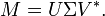
Suppose M is an m-by-n matrix whose entries come from the field K, which is either the field of real numbers or the field of complex numbers. Then there exists a factorization of the form

$M = U\Sigma V^*, \,\!$

where U is an m-by-m unitary matrix over K, the matrix Σ is m-by-n diagonal matrix with nonnegative real numbers on the diagonal, and V* denotes the conjugate transpose of V, an n-by-n unitary matrix over K. Such a factorization is called a singular-value decomposition of M.

A common convention is to order the diagonal entries Σ_i,i in non-increasing fashion. In this case, the diagonal matrix Σ is uniquely determined by M (though the matrices U and V are not). The diagonal entries of Σ are known as the singular values of M.

[edit] Intuitive explanation

In

$M = U\Sigma V^*, \,\!$

the columns of V form a set of orthonormal "input" or "analysing" basis vector directions for M
the columns of U form a set of orthonormal "output" basis vector directions for M
the matrix Σ contains the singular values, which can be thought of as scalar "gain controls" by which each corresponding input is multiplied to give a corresponding output.

[edit] Example

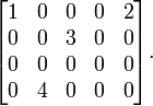
Consider the matrix

$\begin{bmatrix} 1 & 0 & 0 & 0 & 2\\ 0 & 0 & 3 & 0 & 0\\ 0 & 0 & 0 & 0 & 0\\ 0 & 4 & 0 & 0 & 0\end{bmatrix}.$

A singular value decomposition of this matrix is given by

$U = \begin{bmatrix} 0 & 0 & 1 & 0\\ 0 & 1 & 0 & 0\\ 0 & 0 & 0 & -1\\ 1 & 0 & 0 & 0\end{bmatrix} , \Sigma = \begin{bmatrix} 4 & 0 & 0 & 0 & 0\\ 0 & 3 & 0 & 0 & 0\\ 0 & 0 & \sqrt{5} & 0 & 0\\ 0 & 0 & 0 & 0 & 0\end{bmatrix} , V^* = \begin{bmatrix} 0 & 1 & 0 & 0 & 0\\ 0 & 0 & 1 & 0 & 0\\ \sqrt{0.2} & 0 & 0 & 0 & \sqrt{0.8}\\ 0 & 0 & 0 & 1 & 0\\ -\sqrt{0.8} & 0 & 0 & 0 & \sqrt{0.2}\end{bmatrix}$

that is

$\begin{bmatrix} 1 & 0 & 0 & 0 & 2\\ 0 & 0 & 3 & 0 & 0\\ 0 & 0 & 0 & 0 & 0\\ 0 & 4 & 0 & 0 & 0\end{bmatrix} = \begin{bmatrix} 0 & 0 & 1 & 0\\ 0 & 1 & 0 & 0\\ 0 & 0 & 0 & -1\\ 1 & 0 & 0 & 0\end{bmatrix} \cdot \begin{bmatrix} 4 & 0 & 0 & 0 & 0\\ 0 & 3 & 0 & 0 & 0\\ 0 & 0 & \sqrt{5} & 0 & 0\\ 0 & 0 & 0 & 0 & 0\end{bmatrix} \cdot \begin{bmatrix} 0 & 1 & 0 & 0 & 0\\ 0 & 0 & 1 & 0 & 0\\ \sqrt{0.2} & 0 & 0 & 0 & \sqrt{0.8}\\ 0 & 0 & 0 & 1 & 0\\ -\sqrt{0.8} & 0 & 0 & 0 & \sqrt{0.2}\end{bmatrix}$

Notice above that $Σ$ has non-zero values only in its diagonal. Furthermore, because the matrices $U$ and $V *$ are unitary, multiplying by their respective transpose yields the identity matrix, as shown below. In this case, because $U$ and $V *$ are real valued, they each are an orthogonal matrix.

$\begin{bmatrix} 0 & 0 & 1 & 0\\ 0 & 1 & 0 & 0\\ 0 & 0 & 0 & -1\\ 1 & 0 & 0 & 0\end{bmatrix} \cdot \begin{bmatrix} 0 & 0 & 0 & 1\\ 0 & 1 & 0 & 0\\ 1 & 0 & 0 & 0\\ 0 & 0 & -1 & 0\end{bmatrix} = \begin{bmatrix} 1 & 0 & 0 & 0\\ 0 & 1 & 0 & 0\\ 0 & 0 & 1 & 0\\ 0 & 0 & 0 & 1\end{bmatrix}$

and

$\begin{bmatrix} 0 & 0 & \sqrt{0.2} & 0 & -\sqrt{0.8}\\ 1 & 0 & 0 & 0 & 0\\ 0 & 1 & 0 & 0 & 0\\ 0 & 0 & 0 & 1 & 0\\ 0 & 0 & \sqrt{0.8} & 0 & \sqrt{0.2} \end{bmatrix} \cdot \begin{bmatrix} 0 & 1 & 0 & 0 & 0\\ 0 & 0 & 1 & 0 & 0\\ \sqrt{0.2} & 0 & 0 & 0 & \sqrt{0.8}\\ 0 & 0 & 0 & 1 & 0\\ -\sqrt{0.8} & 0 & 0 & 0 & \sqrt{0.2}\end{bmatrix} = \begin{bmatrix} 1 & 0 & 0 & 0 & 0\\ 0 & 1 & 0 & 0 & 0\\ 0 & 0 & 1 & 0 & 0\\ 0 & 0 & 0 & 1 & 0\\ 0 & 0 & 0 & 0 & 1\end{bmatrix}$

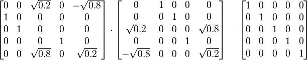
It should also be noted that this singular value decomposition is not unique. For example, choosing $V$ such that

$V^* = \begin{bmatrix} 0 & 1 & 0 & 0 & 0\\ 0 & 0 & 1 & 0 & 0\\ \sqrt{0.2} & 0 & 0 & 0 & \sqrt{0.8}\\ \sqrt{0.4} & 0 & 0 & \sqrt{0.5} & -\sqrt{0.1}\\ -\sqrt{0.4} & 0 & 0 & \sqrt{0.5} & \sqrt{0.1} \end{bmatrix}$

is also a valid singular value decomposition

[edit] Singular values, singular vectors, and their relation to the SVD

A non-negative real number σ is a singular value for M if and only if there exist unit-length vectors u in K^m and v in Kⁿ such that

$Mv = \sigma u \,\mbox{ and } M^{*} u = \sigma v. \,\!$

The vectors u and v are called left-singular and right-singular vectors for σ, respectively.

In any singular value decomposition

$M = U\Sigma V^{*} \,\!$

the diagonal entries of Σ are necessarily equal to the singular values of M. The columns of U and V are, respectively, left- and right-singular vectors for the corresponding singular values. Consequently, the above theorem states that

An m × n matrix M has at least one and at most p = min(m,n) distinct singular values.

It is always possible to find a unitary basis for K^m consisting of left-singular vectors of M.

It is always possible to find a unitary basis for Kⁿ consisting of right-singular vectors of M.

A singular value for which we can find two left (or right) singular vectors that are linearly independent is called degenerate.

Non-degenerate singular values always have unique left and right singular vectors, up to multiplication by a unit phase factor e^iφ (for the real case up to sign). Consequently, if all singular values of M are non-degenerate and non-zero, then its singular value decomposition is unique, up to multiplication of a column of U by a unit phase factor and simultaneous multiplication of the corresponding column of V by the same unit phase factor.

Degenerate singular values, by definition, have non-unique singular vectors. Furthermore, if u₁ and u₂ are two left-singular vectors which both correspond to the singular value σ, then any normalized linear combination of the two vectors is also a left singular vector corresponding to the singular value σ. The similar statement is true for right singular vectors. Consequently, if M has degenerate singular values, then its singular value decomposition is not unique.

[edit] Applications of the SVD

[edit] Pseudoinverse

The singular value decomposition can be used for computing the pseudoinverse of a matrix. Indeed, the pseudoinverse of the matrix M with singular value decomposition $M = U Σ V *$ is

$M^+ = V \Sigma^+ U^*, \,$

where Σ⁺ is the pseudoinverse of Σ, which is formed by replacing every nonzero entry by its reciprocal. The pseudoinverse is one way to solve linear least squares problems.

[edit] Solving homogeneous linear equations

A set of homogeneous linear equations can be written as $\mathbf{A} \, \mathbf{x} = \mathbf{0}$ for a matrix $\mathbf{A}$ and vector $\mathbf{x}$ . A typical situation is that $\mathbf{A}$ is known and a non-zero $\mathbf{x}$ is to be determined which satisfies the equation. Such a $\mathbf{x}$ belongs to $\mathbf{A}$ 's null space and is sometimes called a (right) null vector of $\mathbf{A}$ . $\mathbf{x}$ can be characterized as a right singular vector corresponding to a singular value of $\mathbf{A}$ that is zero. This observation means that if $\mathbf{A}$ has no vanishing singular value, the equation has no non-zero $\mathbf{x}$ as a solution. It also means that if there are several vanishing singular values, any linear combination of the corresponding right singular vectors is a valid solution. Analogously to the definition of a (right) null vector, a non-zero $\mathbf{x}$ satisfying $\mathbf{x}^* \, \mathbf{A} = \mathbf{0}$ , with $\mathbf{x}^*$ denoting the conjugate transpose of $\mathbf{x}$ , is called a left null vector of $\mathbf{A}$ .

[edit] Total least squares minimization

A total least squares problem refers to determining the vector $\mathbf{x}$ which minimizes the 2-norm of a vector $\mathbf{A} \, \mathbf{x}$ under the constraint $\| \mathbf{x} \| = 1$ . The solution turns out to be the right singular vector of $\mathbf{A}$ corresponding to the smallest singular value.

[edit] Range, null space and rank

Another application of the SVD is that it provides an explicit representation of the range and null space of a matrix M. The right singular vectors corresponding to vanishing singular values of M span the null space of M. The left singular vectors corresponding to the non-zero singular values of M span the range of M. As a consequence, the rank of M equals the number of non-zero singular values which is the same as the number of non-zero elements in $Σ$ .

In numerical linear algebra the singular values can be used to determine the effective rank of a matrix, as rounding error may lead to small but non-zero singular values in a rank deficient matrix.

[edit] Matrix approximation

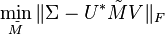
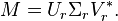
Some practical applications need to solve the problem of approximating a matrix $M$ with another matrix $\tilde{M}$ which has a specific rank $r$ . In the case that the approximation is based on minimizing the Frobenius norm of the difference between $M$ and $\tilde{M}$ under the constraint that $\mbox{rank}(\tilde{M}) = r$ it turns out that the solution is given by the SVD of $M$ , namely

$\tilde{M} = U \tilde{\Sigma} V^*$

where $\tilde{\Sigma}$ is the same matrix as $Σ$ except that it contains only the $r$ largest singular values (the other singular values are replaced by zero). This is known as the Eckart–Young theorem, as it was proved by those two authors in 1936 (although it was later found to have been known to earlier authors; see G. W. Stewart, "On the early history of the singular value decomposition," SIAM Review 35, p. 551-556, 1993).

Quick proof: We hope to minimize $\|M - \tilde M\|_F$ subject to $\mbox{rank}(\tilde{M}) = r$ .

Suppose the SVD of $M = U Σ V *$ . Since the Frobenius norm is unitarily invariant, we have an equivalent statement:

$\min_{\tilde M} \|\Sigma - U^* \tilde M V\|_F$

Note that since $Σ$ is diagonal, $U^* \tilde M V$ should be diagonal in order to minimize the Frobenius norm. Remember that the Frobenius norm is the square-root of the summation of the squared modulus of all entries. This implies that $U$ and $V$ are also singular matrices of $\tilde M$ . Thus we can assume that $\tilde M$ to minimize the above statement has the form:

${\tilde M} = U S V^*,$

where $S$ is diagonal. The diagonal entries $s i$ of $S$ are not necessarily ordered as in SVD.

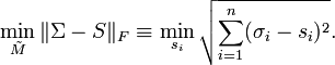
$\min_{\tilde M} \|\Sigma - S\|_F \equiv \min_{s_i} \sqrt {\sum_{i=1}^{n} (\sigma_i - s_i)^2 }.$

From the rank constraint, i.e. $S$ has $r$ non-zero diagonal entries, the minimum of the above statement is obtained as follows:

$\min_{s_i} \sqrt {\sum_{i=1}^{r} (\sigma_i - s_i)^2 + \sum_{i=r+1}^{n} \sigma_i^2 } = \sqrt {\sum_{i=r+1}^{n} \sigma_i^2 }.$

Therefore, $\tilde M$ of rank $r$ is the best approximation of $M$ in the Frobenius norm sense when $\sigma_i = s_i \quad (i=1,\cdots,r)$ and the corresponding singular vectors are same as those of $M$ .

In addition to being the best approximation of a given rank to the matrix under the Frobenius norm, $\tilde M$ as defined above is also the best approximation of that rank under the L₂ norm (see e.g. Trefethen and Bau, Numerical Linear Algebra).

Another example of matrix approximation by SVD is the solution to the orthogonal Procrustes problem of approximating any given matrix by an orthogonal matrix.

[edit] Separable models

The SVD can be thought of as decomposing a matrix into a weighted, ordered sum of separable matrices. By separable, we mean that a matrix $\mathbf{A}$ can be written as an outer product of two vectors $\mathbf{A}= \mathbf{u} \otimes \mathbf{v}$ , or, in coordinates, $\mathbf{A(i,j)}= \mathbf{u}(i) \mathbf{v}(j)$ ; this is also called a simple tensor. Specifically, the matrix M can be decomposed as:

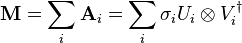
$\mathbf{M} = \sum_i \mathbf{A}_i = \sum_i \sigma_i U_i \otimes V_i ^ \dagger$

Here $U i$ and $V i$ are the i^th columns of the corresponding SVD matrices, $σ i$ are the ordered singular values, and each $\mathbf{A}_i$ is separable. The SVD can be used to find the decomposition of an image processing filter into separable horizontal and vertical filters.^[1] Note that the number of non-zero $σ i$ is exactly the tensor rank: the rank of M, thought of as a tensor.

Separable models often arise in biological systems, and the SVD decomposition is useful to analyze such systems. For example, some visual area V1 simple cells receptive fields can be well described ^[2] by a Gabor filter in the space domain multiplied by a modulation function in the time domain. Thus, given a linear filter evaluated through, for example, reverse correlation, one can rearrange the two spatial dimensions into one dimension, thus yielding a two dimensional filter (space, time) which can be decomposed through SVD. The first column of U in the SVD decomposition is then a Gabor while the first column of V represents the time modulation (or vice-versa). One may then define an index of separability, $\alpha = \sigma_1^2 / \sum_i \sigma_i^2$ , which is the fraction of the power in the matrix M which is accounted for by the first separable matrix in the decomposition ^[3].

[edit] Other examples

The SVD is also applied extensively to the study of linear inverse problems, and is useful in the analysis of regularization methods such as that of Tikhonov. It is widely used in statistics where it is related to principal component analysis, and in signal processing and pattern recognition. It is also used in output-only modal analysis, where the non-scaled mode shapes can be determined from the singular vectors. Yet another usage is latent semantic indexing in natural language text processing.

The SVD also plays a crucial role in the field of Quantum information, in a form often referred to as the Schmidt decomposition. Through it, states of two quantum systems are naturally decomposed, providing a necessary and sufficient condition for them to be entangled : if the rank of the $Σ$ matrix is larger than one.

One application of SVD to rather large matrices is in numerical weather prediction, where Lanczos methods are used to estimate the most linearly quickly growing few perturbations to the central numerical weather prediction over a given initial forward time period — i.e. the singular vectors corresponding to the largest singular values of the linearised propagator for the global weather over that time interval. The output singular vectors in this case are entire weather systems! These perturbations are then run through the full nonlinear model to generate an ensemble forecast, giving a handle on some of the uncertainty that should be allowed for around the current central prediction.

[edit] Relation to eigenvalue decomposition

The singular value decomposition is very general in the sense that it can be applied to any m × n matrix. The eigenvalue decomposition, on the other hand, can only be applied to certain classes of square matrices. Nevertheless, the two decompositions are related.

Given an SVD of M, as described above, the following two relations hold:

$M^{*} M = V \Sigma^{*} U^{*}\, U \Sigma V^{*} = V (\Sigma^{*} \Sigma) V^{*}\,$

$M M^{*} = U \Sigma V^{*} \, V \Sigma^{*} U^{*} = U (\Sigma \Sigma^{*}) U^{*}\,$

The right hand sides of these relations describe the eigenvalue decompositions of the left hand sides. Consequently, the squares of the non-zero singular values of M are equal to the non-zero eigenvalues of either $M * M$ or $M M *$ . Furthermore, the columns of U (left singular vectors) are eigenvectors of $M M *$ and the columns of V (right singular vectors) are eigenvectors of $M * M$ .

In the special case that M is a normal matrix, which by definition must be square, the spectral theorem says that it can be unitarily diagonalized using a basis of eigenvectors, so that it can be written $M = U D U *$ for a unitary matrix U and a diagonal matrix D. When M is Hermitian positive semi-definite, the decomposition $M = U D U *$ is also a singular value decomposition. However, the eigenvalue decomposition and the singular value decomposition differ for all other matrices M: the eigenvalue decomposition is $M = U D U - 1$ where U is not necessarily unitary and D is not necessarily positive semi-definite, while the SVD is $M = U Σ V *$ where Σ is a diagonal positive semi-definite, and U and V are unitary matrices that are not necessarily related except through the matrix M.

[edit] Existence

An eigenvalue λ of a matrix is characterized by the algebraic relation M u = λ u. When M is Hermitian, a variational characterization is also available. Let M be a real n × n symmetric matrix. Define f :Rⁿ → R by f(x) = x^T M x. This continuous function attains a maximum at some u when restricted to the closed unit sphere {||x|| ≤ 1}. By the Lagrange multipliers theorem, u necessarily satisfies

$\nabla f = \nabla \; x^T M x = \lambda \cdot \nabla \; x^T x.$

A short calculation shows the above leads to M u = λ u (symmetry of M is needed here). Therefore λ is the largest eigenvalue of M. The same calculation performed on the orthogonal complement of u gives the next largest eigenvalue and so on. The complex Hermitian case is similar; there f(x) = x* M x is a real-valued function of 2n real variables.

Singular values are similar in that they can be described algebraically or from variational principles. Although, unlike the eigenvalue case, Hermiticity, or symmetry, of M is no longer required.

This section gives these two arguments for existence of singular value decomposition.

[edit] Based on the spectral theorem

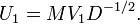
Let M be an m-by-n matrix with complex entries. M*M is positive semidefinite and Hermitian. By the spectral theorem, there exists a unitary n-by-n matrix V such that

$V^* M^* M V = \begin{bmatrix} D & 0 \\ 0 & 0\end{bmatrix}$

where D is diagonal and positive definite. Partition V appropriately so we can write

$\begin{bmatrix} V_1 ^* \\ V_2 ^*\end{bmatrix} M^* M \begin{bmatrix} V_1 & V_2 \end{bmatrix} = \begin{bmatrix} V_1 ^* M^* M V_1 & V_1 ^* M^* M V_2 \\ V_2 ^* M^* M V_1 & V_2 ^* M^* M V_2 \end{bmatrix} = \begin{bmatrix} D & 0 \\ 0 & 0\end{bmatrix}.$

Therefore V*₁M*MV₁ = D, and MV₂ = 0. Define

$U_1 = M V_1 D^{-1/2}.\!$

Then

$U_1 D^{1/2} V_1^* = M V_1 D^{-1/2} D^{1/2} V_1^* = M . \,$

We see that this is almost the desired result, except that U₁ and V₁ are not unitary in general. U₁ is a partial isometry (U₁U*₁ = I ) while V₁ is an isometry (V*₁V₁ = I ). To finish the argument, one simply has to "fill out" these matrices to obtain unitaries. V₂ already does this for V₁. Similarly, one can choose U₂ such that

$U = \begin{bmatrix} U_1 & U_2 \end{bmatrix}$

is unitary.

Define

$\Sigma = \begin{bmatrix} \begin{bmatrix} D^{1/2} & 0 \\ 0 & 0\end{bmatrix} \\ 0 \end{bmatrix}$

where the extra 0 rows are added one row for each column of U₂. Then

$\begin{bmatrix} U_1 & U_2 \end{bmatrix} \begin{bmatrix} \begin{bmatrix} D^{1/2} & 0 \\ 0 & 0\end{bmatrix} \\ 0 \end{bmatrix} \begin{bmatrix} V_1 & V_2 \end{bmatrix}^* = \begin{bmatrix} U_1 & U_2 \end{bmatrix} \begin{bmatrix} D^{1/2} V_1^* \\ 0 \end{bmatrix} = U_1 D^{1/2} V_1^* = M ,$

which is the desired result:

$M = U \Sigma V^* .\!$

Notice the argument could begin with diagonalizing MM* rather than M*M (This shows directly that MM* and M*M have the same non-zero eigenvalues).

[edit] Based on variational characterization

The singular values can also be characterized as the maxima of u^TMv, considered as a function of u and v, over particular subspaces. The singular vectors are the values of u and v where these maxima are attained.

Let M denote an m × n matrix with real entries. Let $S m - 1$ and $S n - 1$ denote the sets of unit 2-norm vectors in R^m and Rⁿ respectively. Define the function

$\sigma(u,v) = u^{T} M v \,$

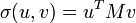
for vectors u ∈ $S m - 1$ and v ∈ $S n - 1$ . Consider the function σ restricted to $S m - 1$ × $S n - 1$ . Since both $S m - 1$ and $S n - 1$ are compact sets, their product is also compact. Furthermore, since σ is continuous, it attains a largest value for at least one pair of vectors u ∈ $S m - 1$ and v ∈ $S n - 1$ . This largest value is denoted σ₁ and the corresponding vectors are denoted u₁ and v₁. Since $σ 1$ is the largest value of $σ(u, v)$ it must be non-negative. If it were negative, changing the sign of either u₁ or v₁ would make it positive and therefore larger.

Statement: u₁, v₁ are left and right singular vectors of M with corresponding singular value σ₁.

Proof: Similar to the eigenvalues case, by assumption the two vectors satisfy the Lagrange multiplier equation:

$\nabla \sigma = \nabla \; u^T M v = \lambda_1 \cdot \nabla \; u^T u + \lambda_2 \cdot \nabla \; v^T v.$

After some algebra, this becomes

$M v_{1} = 2 \lambda_{1} u_{1} + 0, \,$

and

$M^{T} u_{1} = 0 + 2 \lambda_{2} v_{1}. \,$

Multiplying the first equation from left by $u_{1}^{T}$ and the second equation from left by $v_{1}^{T}$ and taking ||u|| = ||v|| = 1 into account gives

$u_{1}^{T} M v_{1} = \sigma_{1} = 2 \lambda_{1},$

$v_{1}^{T} M^{T} u_{1} = \sigma_{1} = 2 \lambda_{2}.$

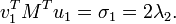
So σ₁ = 2 λ₁ = 2 λ₂. By properties of the functional φ defined by

$\phi(w) = u_1 ^T w, \,$

we have

$M v_{1} = \sigma_{1} u_{1}. \,$

Similarly,

$M^{T} u_{1} = \sigma_{1} v_{1}. \,$

This proves the statement.

More singular vectors and singular values can be found by maximizing σ(u, v) over normalized u, v which are orthogonal to u₁ and v₁, respectively.

The passage from real to complex is similar to the eigenvalue case.

[edit] Geometric meaning

Because U and V are unitary, we know that the columns u₁,...,u_m of U yield an orthonormal basis of K^m and the columns v₁,...,v_n of V yield an orthonormal basis of Kⁿ (with respect to the standard scalar products on these spaces).

The linear transformation T :Kⁿ → K^m that takes a vector x to Mx has a particularly simple description with respect to these orthonormal bases: we have T(v_i) = σ_i u_i, for i = 1,...,min(m,n), where σ_i is the i-th diagonal entry of Σ, and T(v_i) = 0 for i > min(m,n).

The geometric content of the SVD theorem can thus be summarized as follows: for every linear map T :Kⁿ → K^m one can find orthonormal bases of Kⁿ and K^m such that T maps the i-th basis vector of Kⁿ to a non-negative multiple of the i-th basis vector of K^m, and sends the left-over basis vectors to zero. With respect to these bases, the map T is therefore represented by a diagonal matrix with non-negative real diagonal entries.

To get a more visual flavour of singular values and SVD decomposition —at least when working on real vector spaces— consider the sphere S of radius one in Rⁿ. The linear map T maps this sphere onto an ellipsoid in R^m. Non-zero singular values are simply the lengths of the semi-axes of this ellipsoid. Especially when n=m, and all the singular values are distinct and non-zero, the SVD decomposition of the linear map T can be easily analysed as a succession of three consecutive moves : consider the ellipsoid T(S) and specifically its axes ; then consider the directions in Rⁿ sent by T onto these axes. These directions happen to be mutually orthogonal. Apply first an isometry v* sending these directions to the coordinate axes of Rⁿ. On a second move, apply an endomorphism d diagonalized along the coordinate axes and stretching or shrinking in each direction, using the semi-axes lengths of T(S) as stretching coefficients. The composition d o v* then sends the unit-sphere onto an ellipsoid isometric to T(S). To define the third and last move u, just apply an isometry to this ellipsoid so as to carry it over T(S). As can be easily checked, the composition u o d o v* coincides with T.

[edit] Calculating the SVD

The SVD of a matrix M is typically computed by a two-step procedure. In the first step, the matrix is reduced to a bidiagonal matrix. This takes O(mn²) flops, assuming that m ≥ n (this formulation uses the big O notation). The second step is to compute the SVD of the bidiagonal matrix. This step can only be done with an iterative method, so the second step is in principle infinite (just as for eigenvalue algorithms). However, in practice it suffices to compute the SVD up to a certain precision, like the machine epsilon. If this precision is considered constant, then the second step takes O(n) iterations, each costing O(n) flops. Thus, the first step is more expensive, and the overall cost is O(mn²) flops (Bau III & Trefethen 1997, Lecture 31).

The first step can be done using Householder reflections for a cost of 4mn² − 4n³/3 flops, assuming that only the singular values are needed and not the singular vectors. If m is much larger than n then it is advantageous to first reduce the matrix M to a triangular matrix with the QR decomposition and then use Householder reflections to further reduce the matrix to bidiagonal form; the combined cost is 2mn² + 2n³ flops (Bau III & Trefethen 1997, Lecture 31).

The second step can be done by a variant of the QR algorithm for the computation of eigenvalues, which was first described by Golub & Kahan (1965). The LAPACK subroutine DBDSQR implements this iterative method, with some modifications to cover the case the singular values are very small (Demmel & Kahan 1990). Together with a first step using Householder reflections and, if appropriate, QR decomposition, this forms the DGESVD routine for the computation of the singular value decomposition.

The same algorithm is implemented in the GNU Scientific Library (GSL). The GSL also offers an alternative method, which uses a one-sided Jacobi orthogonalization in step 2 (GSL Team 2007). This method computes the SVD of the bidiagonal matrix by solving a sequence of 2-by-2 SVD problems, similar to how the Jacobi eigenvalue algorithm solves a sequence of 2-by-2 eigenvalue methods (Golub & Van Loan 1996, §8.6.3). Yet another method for step 2 uses the idea of divide-and-conquer eigenvalue algorithms (Bau III & Trefethen 1997, Lecture 31).

[edit] Reduced SVDs

In applications it is quite unusual for the full SVD, including a full unitary decomposition of the null-space of the matrix, to be required. Instead, it is often sufficient (as well as faster, and more economical for storage) to compute a reduced version of the SVD. The following can be distinguished for an m×n matrix M of rank r:

[edit] Thin SVD

$M = U_n \Sigma_n V^{*}. \,$

Only the n column vectors of U corresponding to the row vectors of V* are calculated. The remaining column vectors of U are not calculated. This is significantly quicker and more economical than the full SVD if n<<m. The matrix U_n is thus m×n, Σ_n is n×n diagonal, and V is n×n.

The first stage in the calculation of a thin SVD will usually be a QR decomposition of M, which can make for a significantly quicker calculation if n<<m.

[edit] Compact SVD

$M = U_r \Sigma_r V_r^*.$

Only the r column vectors of U and r row vectors of V* corresponding to the non-zero singular values Σ_r are calculated. The remaining vectors of U and V* are not calculated. This is quicker and more economical than the thin SVD if r<<n. The matrix U_r is thus m×r, Σ_r is r×r diagonal, and V_r* is r×n.

[edit] Truncated SVD

$\tilde{M} = U_t \Sigma_t V_t^*.$

Only the t column vectors of U and t row vectors of V* corresponding to the t largest singular values Σ_r are calculated. The rest of the matrix is discarded. This can be much quicker and more economical than the thin SVD if t<<r. The matrix U_t is thus m×t, Σ_t is t×t diagonal, and V_t* is t×n'.

Of course the truncated SVD is no longer an exact decomposition of the original matrix M, but as discussed below, the approximate matrix $\tilde{M}$ is in a very useful sense the closest approximation to M that can be achieved by a matrix of rank t.

[edit] Norms

[edit] Ky Fan norms

The sum of the k largest singular values of M is a matrix norm, the Ky Fan k-norm of M.

The first of the Ky Fan norms, the Ky Fan 1-norm is the same as the operator norm of M as a linear operator with respect to the Euclidean norms of K^m and Kⁿ. In other words, the Ky Fan 1-norm is the operator norm induced by the standard l² Euclidean inner product. For this reason, it is also called the operator 2-norm. One can easily verify the relationship between the Ky Fan 1-norm and singular values. It is true in general, for a bounded operator M on (possibly infinite dimensional) Hilbert spaces

$\| M \| = \| M^* M \|^{\frac{1}{2}}.$

But, in the matrix case, M*M^½ is a normal matrix, so ||M* M||^½ is the largest eigenvalue of M* M^½, i.e. the largest singular value of M.

The last of the Ky Fan norms, the sum of all singular values, is the trace norm, defined by ||M|| = Tr[(M*M)^½] (the diagonal entries of M* M are the squares of the singular values).

[edit] Hilbert-Schmidt norm

The singular values are related to another norm on the space of operators. Consider the Hilbert-Schmidt inner product on the n × n matrices, defined by $\langle M,N\rangle=\operatorname{trace}(M^*N)$ . So the induced norm is $\|M\|=\langle M,M\rangle^{1/2} = \operatorname{trace}(M^*M)^{1/2}$ . Since trace is invariant under unitary equivalence, this shows

$\| M \| = (\sum s_i ^2)^{\frac{1}{2}}$

where s_i are the singular values of M. This is called the Frobenius norm, Schatten 2-norm, or Hilbert-Schmidt norm of M. Direct calculation shows that if

$\, M = (m_{ij}),$

the Frobenius norm of M coincides with

$( \sum_{ij} | m_{ij} | ^2 )^{\frac{1}{2}}.$

[edit] 2DSVD

SVD computes the low-rank approximation of a single matrix (or a set of 1D vectors). This can be generalized to two-dimensional singular value decomposition (2DSVD) to do low-rank approximation of a set of 2D matrices such as a set of images or 2D weather maps.

[edit] HOSVD

Higher order singular value decomposition (HOSVD) is a generalization of SVD for multidimensional arrays (tensors). It is able to give optimal low-rank approximation in given dimensions of a tensor. In the case of a 3 dimensional array (array of matrices) executing HOSVD in 2 dimensions gives the same result as 2DSVD.

[edit] Bounded operators on Hilbert spaces

The factorization $M = U Σ V *$ can be extended to a bounded operator M on a separable Hilbert space H. Namely, for any bounded operator M, there exist a partial isometry U, a unitary V, a measure space (X, μ), and a non-negative measurable f such that

$\; M = U T_f V^*,$

where $T f$ is the multiplication by f on L²(X, μ).

This can be shown by mimicking the linear algebraic argument for the matricial case above. VT_f V* is the unique positive square root of M*M, as given by the Borel functional calculus for self adjoint operators. The reason why U need not be unitary is because, unlike the finite dimensional case, given an isometry U₁ with non trivial kernel, a suitable U₂ may not be found such that

$\begin{bmatrix} U_1 \\ U_2 \end{bmatrix}$

is a unitary operator.

As for matrices, the singular value factorization is equivalent to the polar decomposition for operators: we can simply write

$M = U V^* \cdot V T_f V^*$

and notice that U V* is still a partial isometry while VT_f V* is positive.

[edit] Singular values and compact operators

To extend notion of singular values and left/right-singular eigenvectors to the operator case, one needs to restrict to compact operators. It is a general fact that compact operators on Banach spaces, therefore Hilbert spaces, have only discrete spectrum: If T is compact, every nonzero λ in its spectrum is an eigenvalue. Furthermore, a compact self adjoint operator can be diagonalized by its eigenvectors. If M is compact, so is M*M. Applying the diagonalization result, the unitary image of its positive square root T_f has a set of orthonormal eigenvectors {e_i} corresponding to strictly positive eigenvalues {σ_i}. For any ψ ∈ H,

$\; M \psi = U T_f V^* \psi = \sum_i \langle U T_f V^* \psi, U e_i \rangle U e_i = \sum_i \sigma_i \langle \psi, V e_i \rangle U e_i,$

where the series converges in the norm topology on H. Notice how this resembles the expression from the finite dimensional case. The σ_i 's are called the singular values of M. {U e_i} and {V e_i} can be considered the left- and right-singular vectors of M respectively.

Compact operators on a Hilbert space are the closure of finite rank operators in the uniform operator topology. The above series expression gives an explicit such representation. An immediate consequence of this is:

Theorem M is compact if and only if M*M is compact.

[edit] History

The singular value decomposition was originally developed by differential geometers, who wished to determine whether a real bilinear form could be made equal to another by independent orthogonal transformations of the two spaces it acts on. Eugenio Beltrami and Camille Jordan discovered independently, in 1873 and 1874 respectively, that the singular values of the bilinear forms, represented as a matrix, form a complete set of invariants for bilinear forms under orthogonal substitutions. James Joseph Sylvester also arrived at the singular value decomposition for real square matrices in 1889, apparently independent of both Beltrami and Jordan. Sylvester called the singular values the canonical multipliers of the matrix A. The fourth mathematician to discover the singular value decomposition independently is Autonne in 1915, who arrived at it via the polar decomposition. The first proof of the singular value decomposition for rectangular and complex matrices seems to be by Eckart and Young in 1936; they saw it as a generalization of the principal axis transformation for Hermitian matrices.

In 1907, Erhard Schmidt defined an analog of singular values for integral operators (which are compact, under some weak technical assumptions); it seems he was unaware of the parallel work on singular values of finite matrices. This theory was further developed by Émile Picard in 1910, who is the first to call the numbers $σ k$ singular values (or rather, valeurs singulières).

Practical methods for computing the SVD date back to Kogbetliantz in 1954, 1955 and Hestenes in 1958 resembling closely the Jacobi eigenvalue algorithm, which uses plane rotations or Givens rotations. However, these were replaced by the method of Gene Golub and William Kahan published in 1965 (Golub & Kahan 1965), which uses Householder transformations or reflections. In 1970, Golub and Christian Reinsch published a variant of the Golub/Kahan algorithm that is still the one most-used today.

[edit] See also

[edit] Notes

^ Separable convolution: Part 2 | Steve on Image Processing
^ DeAngelis et al., Receptive-field dynamics in the central visual pathways, Trends Neurosci. 1995, Entrez Pubmed 8545912
^ Depireux et al., Spectro-temporal response field characterization with dynamic ripples in ferret primary auditory cortex, J. Neurophysiol. 2001, Entrez Pubmed 11247991

[edit] References

Bau III, David; Trefethen, Lloyd N. (1997), Numerical linear algebra, Philadelphia: Society for Industrial and Applied Mathematics, ISBN 978-0-89871-361-9 .
Demmel, James; Kahan, William (1990), "Accurate singular values of bidiagonal matrices", Society for Industrial and Applied Mathematics. Journal on Scientific and Statistical Computing 11 (5): 873–912, doi:10.1137/0911052, ISSN 0196-5204 .
Eckart, C., & Young, G. (1936). The approximation of one matrix by another of lower rank. Psychometrika, I, 211-218.
Golub, Gene H.; Kahan, William (1965), "Calculating the singular values and pseudo-inverse of a matrix", Journal of the Society for Industrial and Applied Mathematics: Series B, Numerical Analysis 2 (2): 205–224, http://www.jstor.org/stable/2949777 .
Golub, Gene H.; Van Loan, Charles F. (1996), Matrix Computations (3rd ed.), Johns Hopkins, ISBN 978-0-8018-5414-9 .
GSL Team (2007), "§13.4 Singular Value Decomposition", GNU Scientific Library. Reference Manual .
Halldor, Bjornsson and Venegas, Silvia A. (1997). "A manual for EOF and SVD analyses of climate data". McGill University, CCGCR Report No. 97-1, Montréal, Québec, 52pp.
Hansen, P. C. (1987). The truncated SVD as a method for regularization. BIT, 27, 534-553.
Horn, Roger A. and Johnson, Charles R (1985). "Matrix Analysis". Section 7.3. Cambridge University Press. ISBN 0-521-38632-2.
Horn, Roger A. and Johnson, Charles R (1991). Topics in Matrix Analysis, Chapter 3. Cambridge University Press. ISBN 0-521-46713-6.
Strang G (1998). "Introduction to Linear Algebra". Section 6.7. 3rd ed., Wellesley-Cambridge Press. ISBN 0-9614088-5-5.
Stewart, G. W. (1993), "On the Early History of the Singular Value Decomposition", SIAM Review 35 (4): 551–566, doi:10.1137/1035134, http://citeseer.ist.psu.edu/stewart92early.html .
Wall, Michael E., Andreas Rechtsteiner, Luis M. Rocha (2003). "Singular value decomposition and principal component analysis". in A Practical Approach to Microarray Data Analysis. D.P. Berrar, W. Dubitzky, M. Granzow, eds. pp. 91-109, Kluwer: Norwell, MA.

[edit] External links

[edit] Implementations

[edit] Libraries that support complex and real SVD

LAPACK (website), the Linear Algebra Package. The user manual gives details of subroutines to calculate the SVD (see also [1]).

[edit] Libraries that support real SVD

GNU Scientific Library (website), a numerical C/C++ library supporting SVD (see [2]).
Eigen2, a C++ open source library supporting SVD with an elegant API. It is released under licences LGPL3+ or LGPL2+.
ALGLIB, includes a partial port of the LAPACK to C++, C#, Delphi, Visual Basic, etc.
JAMA, a Java matrix package provided by the NIST.
PROPACK, computes the SVD of large and sparse or structured matrices.
SVDPACK, a library in ANSI FORTRAN 77 implementing four iterative SVD methods. Includes C and C++ interfaces.
SVDLIBC, re-writing of SVDPACK in C.
SVD-Python, pure Python SVD under GNU GPL.
NumPy SVD part of the linalg module of the NumPy module for numerical computing in Python

[edit] Texts and demonstrations

MIT Lecture series by Gilbert Strang. See Lecture #29 on the SVD (scroll down to the bottom till you see "Singular Value Decomposition"). The first 17 minutes give the overview. Then Prof. Strang works two examples. Then the last 4 minutes (min 36 to min 40) are a summary. You can probably fast forward the examples, but the first and last are an excellent concise visual presentation of the topic.
Applications of SVD on PC Hansen's web site.
Introduction to the Singular Value Decomposition by Todd Will of the University of Wisconsin--La Crosse. This site has animations for the visual minded as well as demonstrations of compression using SVD.
Los Alamos group's book chapter has helpful gene data analysis examples.
SVD, another explanation of singular value decomposition
SVD Tutorial,yet another explanation of SVD. Very intuitive.
Javascript script demonstrating the SVD more extensively, paste your data from a spreadsheet.
Javascript script version 2 demonstrating the SVD featere AI-porperties to make a decision support.
Chapter from "Numerical Recipes in C" gives more information about implementation and applications of SVD. (Acrobat DRM plug-in required)
Online Matrix Calculator Performs singular value decomposition of matrices.
A simple tutorial on SVD and applications of Spectral Methods
Matrix and Tensor Decompositions in Genomic Signal Processing
SVD on MathWorld, with image compression as an example application.
If you liked this... New York Times article on SVD in movie-ratings and Netflix

[0] Separable convolution: Part 2 | Steve on Image Processing

[1] DeAngelis et al., Receptive-field dynamics in the central visual pathways, Trends Neurosci. 1995, Entrez Pubmed 8545912

[2] Depireux et al., Spectro-temporal response field characterization with dynamic ripples in ferret primary auditory cortex, J. Neurophysiol. 2001, Entrez Pubmed 11247991

[1]

[2]

[3]