Naive Bayes classifier
From Wikipedia, the free encyclopedia
A naive Bayes classifier is a term in Bayesian statistics dealing with a simple probabilistic classifier based on applying Bayes' theorem with strong (naive) independence assumptions. A more descriptive term for the underlying probability model would be "independent feature model".
In simple terms, a naive Bayes classifier assumes that the presence (or absence) of a particular feature of a class is unrelated to the presence (or absence) of any other feature. For example, a fruit may be considered to be an apple if it is red, round, and about 4" in diameter. Even though these features depend on the existence of the other features, a naive Bayes classifier considers all of these properties to independently contribute to the probability that this fruit is an apple.
Depending on the precise nature of the probability model, naive Bayes classifiers can be trained very efficiently in a supervised learning setting. In many practical applications, parameter estimation for naive Bayes models uses the method of maximum likelihood; in other words, one can work with the naive Bayes model without believing in Bayesian probability or using any Bayesian methods.
In spite of their naive design and apparently over-simplified assumptions, naive Bayes classifiers often work much better in many complex real-world situations than one might expect. Recently, careful analysis of the Bayesian classification problem has shown that there are some theoretical reasons for the apparently unreasonable efficacy of naive Bayes classifiers (Zhang04). An advantage of the naive Bayes classifier is that it requires a small amount of training data to estimate the parameters (means and variances of the variables) necessary for classification. Because independent variables are assumed, only the variances of the variables for each class need to be determined and not the entire covariance matrix.
Contents |
[edit] The naive Bayes probabilistic model
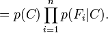
Abstractly, the probability model for a classifier is a conditional model
over a dependent class variable C with a small number of outcomes or classes, conditional on several feature variables F1 through Fn. The problem is that if the number of features n is large or when a feature can take on a large number of values, then basing such a model on probability tables is infeasible. We therefore reformulate the model to make it more tractable.
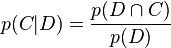
Using Bayes' theorem, we write
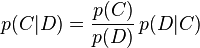
In plain English the above equation can be written as

In practice we are only interested in the numerator of that fraction, since the denominator does not depend on C and the values of the features Fi are given, so that the denominator is effectively constant. The numerator is equivalent to the joint probability model

which can be rewritten as follows, using repeated applications of the definition of conditional probability:


and so forth. Now the "naive" conditional independence assumptions come into play: assume that each feature Fi is conditionally independent of every other feature Fj for  . This means that
and so the joint model can be expressed as

This means that under the above independence assumptions, the conditional distribution over the class variable C can be expressed like this:
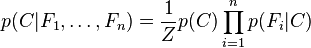
where Z is a scaling factor dependent only on  , i.e., a constant if the values of the feature variables are known.
Models of this form are much more manageable, since they factor into a so-called class prior p(C) and independent probability distributions  . If there are k classes and if a model for p(Fi) can be expressed in terms of r parameters, then the corresponding naive Bayes model has (k − 1) + n r k parameters. In practice, often k = 2 (binary classification) and r = 1 (Bernoulli variables as features) are common, and so the total number of parameters of the naive Bayes model is 2n + 1, where n is the number of binary features used for prediction.
[edit] Parameter estimation
All model parameters (i.e., class priors and feature probability distributions) can be approximated with relative frequencies from the training set. These are maximum likelihood estimates of the probabilities. Non-discrete features need to be discretized first. Discretization can be unsupervised (ad-hoc selection of bins) or supervised (binning guided by information in training data).
If a given class and feature value never occur together in the training set then the frequency-based probability estimate will be zero. This is problematic since it will wipe out all information in the other probabilities when they are multiplied. It is therefore often desirable to incorporate a small-sample correction in all probability estimates such that no probability is ever set to be exactly zero.
[edit] Constructing a classifier from the probability model
The discussion so far has derived the independent feature model, that is, the naive Bayes probability model. The naive Bayes classifier combines this model with a decision rule. One common rule is to pick the hypothesis that is most probable; this is known as the maximum a posteriori or MAP decision rule. The corresponding classifier is the function classify defined as follows:

[edit] Discussion
One should notice that the independence assumption may lead to some unexpected results in the calculation of the posterior probability. In some circumstances, when there is a dependency between observations, the value computed above may be greater than one thereby contradicting the second axiom of probability which requires all probability values to be less than or equal to one.
Despite the fact that the far-reaching independence assumptions are often inaccurate, the naive Bayes classifier has several properties that make it surprisingly useful in practice. In particular, the decoupling of the class conditional feature distributions means that each distribution can be independently estimated as a one dimensional distribution. This in turn helps to alleviate problems stemming from the curse of dimensionality, such as the need for data sets that scale exponentially with the number of features. Like all probabilistic classifiers under the MAP decision rule, it arrives at the correct classification as long as the correct class is more probable than any other class; hence class probabilities do not have to be estimated very well. In other words, the overall classifier is robust enough to ignore serious deficiencies in its underlying naive probability model. Other reasons for the observed success of the naive Bayes classifier are discussed in the literature cited below.
[edit] Example: document classification
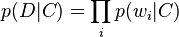
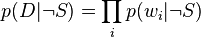
Here is a worked example of naive Bayesian classification to the document classification problem. Consider the problem of classifying documents by their content, for example into spam and non-spam E-mails. Imagine that documents are drawn from a number of classes of documents which can be modelled as sets of words where the (independent) probability that the i-th word of a given document occurs in a document from class C can be written as

(For this treatment, we simplify things further by assuming that the probability of a word in a document is independent of the length of a document, or that all documents are of the same length.)
Then the probability of a given document D, given a class C, is
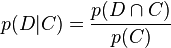
The question that we desire to answer is: "what is the probability that a given document D belongs to a given class C?" In other words, what is  ?
?
Now, by their definition, (see Probability axiom)
and
Bayes' theorem manipulates these into a statement of probability in terms of likelihood.
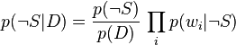
Assume for the moment that there are only two classes, S and ¬S (e.g. spam and not spam).
and
Using the Bayesian result above, we can write:
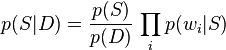
Dividing one by the other gives:
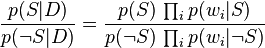
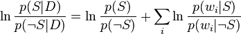
Which can be re-factored as:
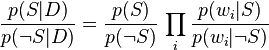
Thus, the probability ratio p(S | D) / p(¬S | D) can be expressed in terms of a series of likelihood ratios. The actual probability p(S | D) can be easily computed from log (p(S | D) / p(¬S | D)) based on the observation that p(S | D) + p(¬S | D) = 1.
Taking the logarithm of all these ratios, we have:
(This technique of "log-likelihood ratios" is a common technique in statistics. In the case of two mutually exclusive alternatives (such as this example), the conversion of a log-likelihood ratio to a probability takes the form of a sigmoid curve: see logit for details.)
Finally, the document can be classified as follows. It is spam if 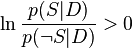 , otherwise it is not spam.
[edit] See also
- Bayesian spam filtering
- Bayesian network
- Random naive Bayes
- Linear classifier
- Bayesian inference (esp. as Bayesian techniques relate to spam)
- Boosting
- Fuzzy logic
- Logistic regression
- Neural networks
- Predictive analytics
- Perceptron
- Support vector machine
[edit] References
- Domingos, Pedro & Michael Pazzani (1997) "On the optimality of the simple Bayesian classifier under zero-one loss". Machine Learning, 29:103–137. (also online at CiteSeer: [1])
- Rish, Irina. (2001). "An empirical study of the naive Bayes classifier". IJCAI 2001 Workshop on Empirical Methods in Artificial Intelligence. (available online: PDF, PostScript)
- Hand, DJ, & Yu, K. (2001). "Idiot's Bayes - not so stupid after all?" International Statistical Review. Vol 69 part 3, pages 385-399. ISSN 0306-7734.
- Mozina M, Demsar J, Kattan M, & Zupan B. (2004). "Nomograms for Visualization of Naive Bayesian Classifier". In Proc. of PKDD-2004, pages 337-348. (available online: PDF)
- Maron, M. E. (1961). "Automatic Indexing: An Experimental Inquiry." Journal of the ACM (JACM) 8(3):404–417. (available online: PDF)
- Minsky, M. (1961). "Steps toward Artificial Intelligence." Proceedings of the IRE 49(1):8-30.
- McCallum, A. and Nigam K. "A Comparison of Event Models for Naive Bayes Text Classification". In AAAI/ICML-98 Workshop on Learning for Text Categorization, pp. 41-48. Technical Report WS-98-05. AAAI Press. 1998. (available online: PDF)
- Harry Zhang "The Optimality of Naive Bayes". (available online: PDF)
- S.Kotsiantis, P. Pintelas, Increasing the Classification Accuracy of Simple Bayesian Classifier, Lecture Notes in Artificial Intelligence, AIMSA 2004, Springer-Verlag Vol 3192, pp. 198-207, 2004 (http://www.math.upatras.gr/~esdlab/en/members/kotsiantis/improvingNB.pdf)
- S. Kotsiantis, P. Pintelas, Logitboost of Simple Bayesian Classifier, Computational Intelligence in Data mining Special Issue of the Informatica Journal, Vol 29 (1), pp. 53-59, 2005 (http://www.math.upatras.gr/~esdlab/en/members/kotsiantis/05_Kotsiantis-Logitboost%20of%20simble%20bayesian..._No%205.pdf)
[edit] External links
- Naive Bayesian learning
- Hierarchical Naive Bayes Classifiers for uncertain data (an extension of the Naive Bayes classifier).
- Online application of a Naive Bayes classifier (emotion modelling), with a full explanation.
- BayesNews - Bayesian RSS Reader (useful for personal news clipping).
- Software
- Naive Bayes implementation in Visual Basic (includes executable and source code).
- An interactive Microsoft Excel spreadsheet Naive Bayes implementation using VBA (requires enabled macros) with viewable source code.
- jBNC - Bayesian Network Classifier Toolbox
- POPFile Perl-based email proxy system classifies email into user-defined "buckets", including spam.
- Statistical Pattern Recognition Toolbox for Matlab.
- Document Classification Using Naive Bayes Classifier with Perl.
- sux0r An Open Source Content management system with a focus on Naive Bayesian categorization and probabilistic content.
- ifile - the first freely available (Naive) Bayesian mail/spam filter
- Naive Bayes algorithm in the Visual Numerics IMSL C Library

