Mahalanobis distance
From Wikipedia, the free encyclopedia
In statistics, Mahalanobis distance is a distance measure introduced by P. C. Mahalanobis in 1936.[1] It is based on correlations between variables by which different patterns can be identified and analyzed. It is a useful way of determining similarity of an unknown sample set to a known one. It differs from Euclidean distance in that it takes into account the correlations of the data set and is scale-invariant, i.e. not dependent on the scale of measurements.
Contents |
[edit] Definition
Formally, the Mahalanobis distance from a group of values with mean  and covariance matrix S for a multivariate vector
  is defined as:

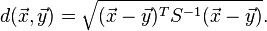
Mahalanobis distance (or "generalized squared interpoint distance" for its squared value[3]) can also be defined as dissimilarity measure between two random vectors  and
and  of the same distribution with the covariance matrix S :
If the covariance matrix is the identity matrix, the Mahalanobis distance reduces to the Euclidean distance. If the covariance matrix is diagonal, then the resulting distance measure is called the normalized Euclidean distance:

where σi is the standard deviation of the xi over the sample set.
[edit] Intuitive explanation
Consider the problem of estimating the probability that a test point in N-dimensional Euclidean space belongs to a set, where we are given sample points that definitely belong to that set. Our first step would be to find the average or center of mass of the sample points. Intuitively, the closer the point in question is to this center of mass, the more likely it is to belong to the set.
However, we also need to know how large the set is. The simplistic approach is to estimate the standard deviation of the distances of the sample points from the center of mass. If the distance between the test point and the center of mass is less than one standard deviation, then we conclude that it is highly probable that the test point belongs to the set. The further away it is, the more likely that the test point should not be classified as belonging to the set.
This intuitive approach can be made quantitative by defining the normalized distance between the test point and the set to be  . By plugging this into the normal distribution we get the probability of the test point belonging to the set.
The drawback of the above approach was that we assumed that the sample points are distributed about the center of mass in a spherical manner. Were the distribution to be decidedly non-spherical, for instance ellipsoidal, then we would expect the probability of the test point belonging to the set to depend not only on the distance from the center of mass, but also on the direction. In those directions where the ellipsoid has a short axis the test point must be closer, while in those where the axis is long the test point can be further away from the center.
Putting this on a mathematical basis, the ellipsoid that best represents the set's probability distribution can be estimated by building the covariance matrix of the samples. The Mahalanobis distance is simply the distance of the test point from the center of mass divided by the width of the ellipsoid in the direction of the test point.
This last property, of minimizing the distance between a test point and the mean, is common to all Bregman divergences, of which the Mahalanobis distance is an example.
[edit] Relationship to leverage
Mahalanobis distance is closely related to the leverage statistic, h, but has a different scale:[4]
- Mahalanobis distance = (N − 1)(h − 1/N).
[edit] Applications
Mahalanobis' discovery was prompted by the problem of identifying the similarities of skulls based on measurements in 1927.[5]
Mahalanobis distance is widely used in cluster analysis and other classification techniques. It is closely related to Hotelling's T-square distribution used for multivariate statistical testing and Fisher's Linear Discriminant Analysis that is used for supervised classification.[6]
In order to use the Mahalanobis distance to classify a test point as belonging to one of N classes, one first estimates the covariance matrix of each class, usually based on samples known to belong to each class. Then, given a test sample, one computes the Mahalanobis distance to each class, and classifies the test point as belonging to that class for which the Mahalanobis distance is minimal. Using the probabilistic interpretation given above, this is equivalent to selecting the class with the maximum likelihood.[citation needed]
Also, Mahalanobis distance and leverage are often used to detect outliers, especially in the development of linear regression models. A point that has a greater Mahalanobis distance from the rest of the sample population of points is said to have higher leverage since it has a greater influence on the slope or coefficients of the regression equation. Mahalanobis distance is also used to determine multivariate outliers. Regression techniques can be used to determine if a specific case within a sample population is an outlier via the combination of two or more variable scores. A case need not be a univariate outlier on a variable to be a multivariate outlier. The significance of a Mahalanobis distance when detecting multivariate outliers is evaluated as a Chi Square with k degrees of freedom.[citation needed]
[edit] References
- ^ Mahalanobis, P C (1936). "On the generalised distance in statistics". Proceedings of the National Institute of Sciences of India 2 (1): 49–55. http://ir.isical.ac.in/dspace/handle/1/1268. Retrieved on 2008-11-05.
- ^ De Maesschalck, R.; D. Jouan-Rimbaud, D.L. Massart (2000) The Mahalanobis distance. Chemometrics and Intelligent Laboratory Systems 50:1–18
- ^ Gnanadesikan, R., and J.R. Kettenring (1972). Robust estimates, residuals, and outlier detection with multiresponse data. Biometrics 28:81-124.
- ^ Schinka, J. A., Velicer, W. F., & Weiner, I. B. (2003). Research methods in psychology. Wiley.
- ^ Mahalanobis, P. C. (1927). Analysis of race mixture in Bengal. J. Proc. Asiatic Soc. of Bengal. 23:301-333.
- ^ McLachlan, Geoffry J (1992) Discriminant Analysis and Statistical Pattern Recognition. Wiley Interscience. ISBN 0471691151 p. 12

