Ohm's law
From Wikipedia, the free encyclopedia

Ohm's law applies to electrical circuits; it states that the current through a conductor between two points is directly proportional to the potential difference or voltage across the two points, and inversely proportional to the resistance between them.
The mathematical equation that describes this relationship is:

where I is the current in amperes, V is the potential difference in volts, and R is a circuit parameter called the resistance (measured in ohms, also equivalent to volts per ampere). The potential difference is also known as the voltage drop, and is sometimes denoted by U, E or emf (electromotive force) instead of V.[1]
The law was named after the German physicist Georg Ohm, who, in a treatise published in 1827, described measurements of applied voltage and current through simple electrical circuits containing various lengths of wire. He presented a slightly more complex equation than the one above to explain his experimental results. The above equation is the modern form of Ohm's law.
The resistance of most resistive devices (resistors) is constant over a large range of values of current and voltage. When a resistor is used under these conditions, the resistor is referred to as an ohmic device (or an ohmic resistor) because a single value for the resistance suffices to describe the resistive behavior of the device over the range. When sufficiently high voltages are applied to a resistor, forcing a high current through it, the device is no longer ohmic because its resistance, when measured under such electrically stressed conditions, is different (typically greater) from the value measured under standard conditions (see temperature effects, below).
Ohm's law, in the form above, is an extremely useful equation in the field of electrical/electronic engineering because it describes how voltage, current and resistance are interrelated on a "macroscopic" level, that is, commonly, as circuit elements in an electrical circuit. Physicists who study the electrical properties of matter at the microscopic level use a closely related and more general vector equation, sometimes also referred to as Ohm's law, having variables that are closely related to the I, V and R scalar variables of Ohm's law, but are each functions of position within the conductor. See the Physics and Relation to heat conduction sections below.
Electrical circuits consist of electrical devices connected by wires (or other suitable conductors). (See the article electrical circuits for some basic combinations.) The above diagram shows one of the simplest electrical circuits that can be constructed. One electrical device is shown as a circle with + and - terminals, which represents a voltage source such as a battery. The other device is illustrated by a zig-zag symbol and has an R beside it. This symbol represents a resistor, and the R designates its resistance. The + or positive terminal of the voltage source is connected to one of the terminals of the resistor using a wire of negligible resistance, and through this wire a current I is shown, in a specified direction illustrated by the arrow. The other terminal of the resistor is connected to the - or negative terminal of the voltage source by a second wire. This configuration forms a complete circuit because all the current that leaves one terminal of the voltage source must return to the other terminal of the voltage source. (While not shown, because electrical engineers assume that it exists, there is an implied current I, and an arrow pointing to the left, associated with the second wire.)
Voltage is the electrical driver that moves (negatively charged) electrons through wires and electrical devices, current is the rate of electron flow, and resistance is the property of a resistor (or other device that obeys Ohm's law) that limits current to an amount proportional to the applied voltage. So, for a given resistance R (ohms), and a given voltage V (volts) established across the resistance, Ohm's law provides the equation (I=V/R) for calculating the current through the resistor (or device).
The "conductor" mentioned by Ohm's law is a circuit element across which the voltage is measured. Resistors are conductors that slow down the passage of electric charge. A resistor with a high value of resistance, say greater than 10 megohms, is a poor conductor, while a resistor with a low value, say less than 0.1 ohm, is a good conductor. (Insulators are materials that, for most practical purposes, do not allow a current when a voltage is applied.)
In a circuit diagram, like the one above, the various components may be joined by connectors, contacts, welds or solder joints of various kinds, but for simplicity these connections are usually not shown.
Contents |
[edit] Physics
Physicists often use the continuum form of Ohm's Law:[2]

where J is the current density (current per unit area, unlike the simpler I, units of amperes, of Ohm's law), σ is the conductivity (which can be a tensor in anisotropic materials) and E is the electric field (units of volts per meter, unlike the simpler V, units of volts, of Ohm's law). While the notation above does not explicitly depict the variables, each are vectors and each are functions of three position variables. That is, in the case of J, using cartesian coordinates, there are actually three separate equations, one for each component of the vector, each equation having three independent position variables. For example, the components of J in the x, y and z directions would be Jx(x,y,z), Jy(x,y,z) and Jz(x,y,z).

The advantage of this form is that it describes electrical behaviour at a single point and does not depend on the geometry of the conductor being considered. It only depends on the material of the conductor which determines the conductivity. That this is a form of Ohm's law can be shown by considering a conductor of length l, uniform cross-sectional area a and a uniform field  applied along its length.
The potential difference between two points is defined as
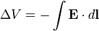
with  the element of path along the integration of electric field vector E. For a uniform applied field and defining the voltage in the usual convention of opposite direction to the field;

Substituting current per unit area, J, for I / a (a being the cross section of the conductor), the continuum form becomes:

The electrical resistance of a uniform conductor is given, in terms of conductivity, by:

After substitution Ohm's law takes on the more familiar, yet macroscopic and averaged version:

A perfect crystal lattice, with low enough thermal motion and no deviations from periodic structure, would have no resistivity,[3] but a real metal has crystallographic defects, impurities, multiple isotopes, and thermal motion of the atoms. Electrons scatter from all of these, resulting in resistance to their flow.
[edit] Magnetic effects
The continuum form of the equation is only valid in the reference frame of the conducting material. If the material is moving at velocity v relative to a magnetic field B, a term must be added as follows:

See Lorentz force for more on this and Hall effect for some other implications of a magnetic field. This equation is not a modification to Ohm's law. Rather, it is analogous in circuit analysis terms to taking into account inductance as well as resistance.
[edit] How electrical engineers use Ohm's law

Ohm's law is one of the basic equations used in the analysis of electrical circuits. It applies to both metal conductors and circuit components (resistors) specifically made for this behaviour. Both are ubiquitous in electrical engineering. Materials and components that obey Ohm's law are described as "ohmic".[4]
There are, however, components of electrical circuits which do not obey Ohm's law; that is, their relationship between current and voltage (their I–V curve) is nonlinear. An example is the p-n junction diode. The ratio V/I is sometimes called the static, or chordal, or DC, resistance.[5][6] However, in some diode applications, the AC signal applied to the device is small and it is possible to analyze the circuit in terms of the dynamic, small-signal, or incremental resistance, defined as the slope of the V–I curve (or inverse slope of the I–V curve, that is, the derivative of current with respect to voltage). For sufficiently small signals, the dynamic resistance allows the Ohm's law proportionality to be applied as an approximation.[7]
[edit] Hydraulic analogies
A hydraulic analogy is sometimes used to describe Ohm's Law. Water pressure, measured by pascals (or PSI), is the analog of voltage because establishing a water pressure difference between two points along a (horizontal) pipe causes water to flow. Water flow rate, as in liters per second, is the analog of current, as in coulombs per second. Finally, flow restrictors — such as apertures placed in pipes between points where the water pressure is measured — are the analog of resistors. We say that the rate of water flow through an aperture restrictor is proportional to the difference in water pressure across the restrictor. Similarly, the rate of flow of electrical charge, that is, the electric current, through an electrical resistor is proportional to the difference in voltage measured across the resistor.
Flow and pressure variables can be calculated in fluid flow network with the use of the hydraulic ohm analogy.[8][9] The method can be applied to both steady and transient flow situations.
[edit] Temperature effects
When the temperature of the conductor increases, the collisions between electrons and ions increase. Thus as a substance heats up because of electricity flowing through it (or by any heating process), the resistance will usually increase. The exception is semiconductors. The resistance of an ohmic substance depends on temperature in the following way:
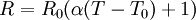
where T is its temperature, T0 is a reference temperature (usually room temperature), R0 is the resistance at T0, and α is the percentage change in resistivity per unit temperature. The constant α depends only on the material being considered. The relationship stated is actually only an approximate one, the true physics being somewhat non-linear, or looking at it another way, α itself varies with temperature. For this reason it is usual to specify the temperature that α was measured at with a suffix, such as α15 and the relationship only holds in a range of temperatures around the reference.[10]
Intrinsic semiconductors exhibit the opposite temperature behavior, becoming better conductors as the temperature increases. This occurs because the electrons are bumped to the conduction energy band by the thermal energy, where they can flow freely and in doing so they leave behind holes in the valence band which can also flow freely.
Extrinsic semiconductors have much more complex temperature behaviour. First the electrons (or holes) leave the donors (or acceptors) giving a decreasing resistance. Then there is a fairly flat phase in which the semiconductor is normally operated where almost all of the donors (or acceptors) have lost their electrons (or holes) but the number of electrons that have jumped right over the energy gap is negligible compared to the number of electrons (or holes) from the donors (or acceptors). Finally as the temperature increases further the carriers that jump the energy gap becomes the dominant figure and the material starts behaving like an intrinsic semiconductor.[11]
[edit] Strain (mechanical) effects
Just as the resistance of a conductor depends upon temperature, the resistance of a conductor depends upon strain. By placing a conductor under tension (a form of stress that leads to strain in the form of stretching of the conductor), the length of the section of conductor under tension increases and its cross-sectional area decreases. Both these effects contribute to increasing the resistance of the strained section of conductor. Under compression (strain in the opposite direction), the resistance of the strained section of conductor decreases. See the discussion on strain gauges for details about devices constructed to take advantage of this effect.
[edit] Transients and AC circuits
Ohm's law holds for linear circuits where the current and voltage are steady (DC), and for instantaneous voltage and current in linear circuits with no reactive elements. When the current and voltage are varying, effects other than resistance may be at work; these effects are principally those of inductance and capacitance. When such reactive elements, or transmission lines, are involved in a circuit, the relationship between voltage and current becomes the solution to a differential equation.
Equations for time-invariant AC circuits take the same form as Ohm's law, however, if the variables are generalized to complex numbers and the current and voltage waveforms are complex exponentials.[12]
In this approach, a voltage or current waveform takes the form Aest, where t is time, s is a complex parameter, and A is a complex scalar. In any linear time-invariant system, all of the currents and voltages can be expressed with the same s parameter as the input to the system, allowing the time-varying complex exponential term to be canceled out and the system described algebraically in terms of the complex scalars in the current and voltage waveforms.
The complex generalization of resistance is impedance, usually denoted Z; it can be shown that for an inductor,

and for a capacitor,

We can now write,

where V and I are the complex scalars in the voltage and current respectively and Z is the complex impedance.
While this has the form of Ohm's law, with Z taking the place of R, it is not the same as Ohm's law. When Z is complex, only the real part is responsible for dissipating heat.
In the general AC circuit, Z will vary strongly with the frequency parameter s, and so also will the relationship between voltage and current.
For the common sinusoidal case, the s parameter is taken to be jω, corresponding to a complex sinusoid Aejωt. The real parts of such complex current and voltage waveforms describe the actual sinusoidal currents and voltages in a circuit, which can be in different phases due to the different complex scalars.
[edit] Relation to heat conduction
Ohm's principle predicts the flow of electrical charge (i.e. current) in electrical conductors when subjected to the influence of voltage differences; Jean-Baptiste-Joseph Fourier's principle predicts the flow of heat in heat conductors when subjected to the influence of temperature differences.
The same equation describes both phenomena, the equation's variables taking on different meanings in the two cases. Specifically, solving a heat conduction (Fourier) problem with temperature (the driving "force") and flux of heat (the rate of flow of the driven "quantity", i.e. heat energy) variables also solves an analogous electrical conduction (Ohm) problem having electric potential (the driving "force") and electric current (the rate of flow of the driven "quantity", i.e. charge) variables.
The basis of Fourier's work was his clear conception and definition of thermal conductivity. He assumed that, all else being the same, the flux of heat is strictly proportional to the gradient of temperature. Although undoubtedly true for small temperature gradients, strictly proportional behavior will be lost when real materials (e.g. ones having a thermal conductivity that is a function of temperature) are subjected to large temperature gradients.
A similar assumption is made in the statement of Ohm's law: other things being alike, the strength of the current at each point is proportional to the gradient of electric potential. The accuracy of the assumption that flow is proportional to the gradient is more readily tested, using modern measurement methods, for the electrical case than for the heat case.
[edit] History
In January 1781, before Georg Ohm's work, Henry Cavendish experimented with Leyden jars and glass tubes of varying diameter and length filled with salt solution. He measured the current by noting how strong a shock he felt as he completed the circuit with his body. Cavendish wrote that the "velocity" (current) varied directly as the "degree of electrification" (voltage). He did not communicate his results to other scientists at the time,[13] and his results were unknown until Maxwell published them in 1879.[14]
Ohm did his work on resistance in the years 1825 and 1826, and published his results in 1827 as the book Die galvanische Kette, mathematisch bearbeite (The galvanic Circuit investigated mathematically).[15] He drew considerable inspiration from Fourier's work on heat conduction in the theoretical explanation of his work. For experiments, he initially used voltaic piles, but later used a thermocouple as this provided a more stable voltage source in terms of internal resistance and constant potential difference. He used a galvanometer to measure current, and knew that the voltage between the thermocouple terminals was proportional to the junction temperature. He then added test wires of varying length, diameter, and material to complete the circuit. He found that his data could be modeled through the equation

where X was the reading from the galvanometer, l was the length of the test conductor, a depended only on the thermocouple junction temperature, and b was a constant of the entire setup. From this, Ohm determined his law of proportionality and published his results.
Ohm's law was probably the most important of the early quantitative descriptions of the physics of electricity. We consider it almost obvious today. When Ohm first published his work, this was not the case; critics reacted to his treatment of the subject with hostility. They called his work a "web of naked fancies"[16] and the German Minister of Education proclaimed that Ohm was "a professor who preached such heresies was unworthy to teach science."[17] The prevailing scientific philosophy in Germany at the time, led by Hegel, asserted that experiments need not be performed to develop an understanding of nature because nature is so well ordered, and that scientific truths may be deduced through reasoning alone. Also, Ohm's brother Martin, a mathematician, was battling the German educational system. These factors hindered the acceptance of Ohm's work, and his work did not become widely accepted until the 1840s. Fortunately, Ohm received recognition for his contributions to science well before he died.
In the 1850s, Ohm's law was known as such, and was widely considered proved, and alternatives such as "Barlow's law" discredited, in terms of real applications to telegraph system design, as discussed by Samuel F. B. Morse in 1855.[18]
While the old term for electrical conductance, the mho (the inverse of the resistance unit ohm), is still used, a new name, the siemens, was adopted in 1971, honoring Ernst Werner von Siemens. The siemens is preferred in formal papers.
In the 1920s, it was discovered that the current through an ideal resistor actually has statistical fluctuations, which depend on temperature, even when voltage and resistance are exactly constant; this fluctuation, now known as Johnson–Nyquist noise, is due to the discrete nature of charge. This thermal effect implies that measurements of current and voltage that are taken over sufficiently short periods of time will yield ratios of V/I that fluctuate from the value of R implied by the time average or ensemble average of the measured current; Ohm's law remains correct for the average current, in the case of ordinary resistive materials.
Ohm's work long preceded Maxwell's equations and any understanding of frequency-dependent effects in AC circuits. Modern developments in electromagnetic theory and circuit theory do not contradict Ohm's law when they are evaluated within the appropriate limits.
[edit] See also
- Poiseuille's law
- Scientific laws named after people
- Ohm's acoustic law
- Hydraulic analogy
- Hopkinson's Law ("Ohm's Law for magnetics")
- Sheet resistance
- Walking along the resistive film - building various resistive circuits by reproducing Ohm's experiment nowadays
[edit] References
- ^ Handbook of Chemistry and Physics, Fortieth Edition, p.3112, 1958
- ^ Seymour J, Physical Electronics, pp 53–54, Pitman, 1972
- ^ Seymour J, Physical Electronics, pp 48–49, Pitman, 1972
- ^ Hughes, E, Electrical Technology, pp10, Longmans, 1969.
- ^ Forbes T. Brown (2006). Engineering System Dynamics. CRC Press. p. 43. ISBN 9780849396489. http://books.google.com/books?id=UzqX4j9VZWcC&pg=PA43&dq=%22chordal+resistance%22&as_brr=3&ei=Z0x0Se2yNZHGlQSpjMyvDg.
- ^ Kenneth L. Kaiser (2004). Electromagnetic Compatibility Handbook. CRC Press. p. 13–52. ISBN 9780849320873. http://books.google.com/books?id=nZzOAsroBIEC&pg=PT1031&dq=%22static+resistance%22+%22dynamic+resistance%22+nonlinear&lr=&as_brr=3&ei=Kk50Ser1MJeOkAS9wNTwDg#PPT1031,M1.
- ^ Horowitz, Paul; Winfield Hill (1989). The Art of Electronics (2nd ed.). Cambridge University Press. p. 13. ISBN 0-521-37095-7. http://books.google.com/books?id=bkOMDgwFA28C&pg=PA13&dq=small-signal+%22dynamic+resistance%22&lr=&as_brr=3&as_pt=ALLTYPES&ei=lrd0SfiSG5HGlQSpjMyvDg.
- ^ A. Akers, M. Gassman, & R. Smith (2006). Hydraulic Power System Analysis. New York: Taylor & Francis. Chapter 13. ISBN 0-8247-9956-9. http://books.google.com/books?id=Uo9gpXeUoKAC&pg=PA299&dq=ohm+intitle:Hydraulic+intitle:Power+intitle:System+intitle:Analysis&lr=&as_brr=0&ei=-jWfSKCaMJCKtAPH_q2eBQ&sig=ACfU3U24HWSO6oF43Z1txszv5fXZR68iFA.
- ^ A. Esposito, "A Simplified Method for Analyzing Circuits by Analogy", Machine Design, October 1969, pp. 173–177.
- ^ Ward, MR, Electrical Engineering Science, pp36–40, McGraw-Hill, 1971.
- ^ Seymour J, Physical Electronics, chapter 2, Pitman, 1972
- ^ Rajendra Prasad (2006). Fundamentals of Electrical Engineering. Prentice-Hall of India. http://books.google.com/books?id=nsmcbzOJU3kC&pg=PA140&dq=ohm%27s-law+complex+exponentials&lr=&as_brr=3&ei=k1rwR4ffNo2AsgPNhtnCBg&sig=mjShqNIvu1F9qL5g7I7ET2JrOg8#PPA138,M1.
- ^ "Electricity". Encyclopedia Britannica. 1911. http://www.1911encyclopedia.org/Electricity.
- ^ Sanford P. Bordeau (1982) Volts to Hertz...the Rise of Electricity. Burgess Publishing Company, Minneapolis, MN. pp.86–107, ISBN 0808749080
- ^ G. S. Ohm (1827). Die galvanische Kette, mathematisch bearbeite. Berlin: T. H. Riemann. http://www.ohm-hochschule.de/bib/textarchiv/Ohm.Die_galvanische_Kette.pdf.
- ^ Davies, B, "A web of naked fancies?", Physics Education 15 57–61, Institute of Physics, Issue 1, Jan 1980 [1]
- ^ Hart, IB, Makers of Science, London, Oxford University Press, 1923. p. 243. [2]
- ^ Taliaferro Preston (1855). Shaffner's Telegraph Companion: Devoted to the Science and Art of the Morse Telegraph. Vol.2. Pudney & Russell. http://books.google.com/books?id=TDEOAAAAYAAJ&pg=RA1-PA43&dq=ohm%27s-law+date:0-1860&lr=&as_brr=1&ei=EljwR83SIJTQtgPvxOmCBw.
[edit] External links
- What are Volts, Amps, Watts etc? – Ohms law and explanations of fundamental electronics principles
- Ohm's law – NASA Glenn Research Center, Learning Technologies Project
- Interactive calculator for Ohm's Law and other circuit parameters – The Electronics Calculator Website
- Interactive simulation – Simple electric circuits Java applet

