Lorenz curve
From Wikipedia, the free encyclopedia
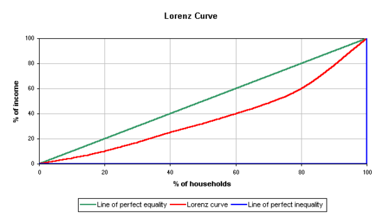
In economics, the Lorenz curve is a graphical representation of the cumulative distribution function of a probability distribution; it is a graph showing the proportion of the distribution assumed by the bottom y% of the values. It is a curve that illustrates income distribution.[1] It is often used to represent income distribution, where it shows for the bottom x% of households, what percentage y% of the total income they have. The percentage of households is plotted on the x-axis, the percentage of income on the y-axis. It can also be used to show distribution of assets. In such use, many economists consider it to be a measure of social inequality. It was developed by Max O. Lorenz in 1905 for representing income distribution.
Contents |
[edit] Explanation
Every point on the Lorenz curve represents a statement like "the bottom 20% of all households have 10% of the total income." A perfectly equal income distribution would be one in which every person has the same income. In this case, the bottom "N"% of society would always have "N"% of the income. This can be depicted by the straight line "y" = "x"; called the "line of perfect equality."
By contrast, a perfectly unequal distribution would be one in which one person has all the income and everyone else has none. In that case, the curve would be at "y" = 0 for all "x" < 100%, and "y" = 100% when "x" = 100%. This curve is called the "line of perfect inequality."
The Gini coefficient is the area between the line of perfect equality and the observed Lorenz curve, as a percentage of the area between the line of perfect equality and the line of perfect inequality. (This equals two times the area between the line of perfect equality and the observed Lorenz curve.) The higher the coefficient, the more unequal the distribution is.
[edit] Calculation
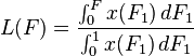
The Lorenz curve can often be represented by a function L(F), where F is represented by the horizontal axis, and L is represented by the vertical axis.
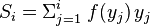
For a population of size n, with a sequence of values yi, i = 1 to n, that are indexed in non-decreasing order ( yi ≤ yi+1), the Lorenz curve is the continuous piecewise linear function connecting the points ( Fi , Li ), i = 0 to n, where F0 = 0, L0 = 0, and for i = 1 to n:


For a discrete probability function f(y), let yi, i = 1 to n, be the points with non-zero probabilities indexed in increasing order ( yi < yi+1). The Lorenz curve is the continuous piecewise linear function connecting the points ( Fi , Li ), i = 0 to n, where F0 = 0, L0 = 0, and for i = 1 to n:

For a probability density function f(x) with the cumulative distribution function F(x), the Lorenz curve L(F(x)) is given by:

For a cumulative distribution function F(x) with inverse x(F), the Lorenz curve L(F) is given by:
The inverse x(F) may not exist because the cumulative distribution function has jump discontinuities or intervals of constant values. However, the previous formula can still apply by generalizing the definition of x(F):
- x(F1) = inf {y : F(y) ≥ F1}
For an example of a Lorenz curve, see Pareto distribution.
[edit] Properties
A Lorenz curve always starts at (0,0) and ends at (1,1).
The Lorenz curve is not defined if the mean of the probability distribution is zero or infinite.
The Lorenz curve for a probability distribution is a continuous function. However, Lorenz curves representing discontinuous functions can be constructed as the limit of Lorenz curves of probability distributions, the line of perfect inequality being an example.
If the variable being measured cannot take negative values, the Lorenz curve:
- cannot rise above the line of perfect equality,
- cannot sink below the line of perfect inequality,
- is increasing, and
- is a convex function.
If the variable being measured can take negative values but has a positive mean, then the Lorenz curve will sink below the line of perfect inequality and is a convex function.
If the variable being measured can take negative values and has a negative mean, then the Lorenz curve will be above the line of perfect equality, except at the end points, and is a concave function.
The Lorenz curve is invariant under positive scaling. If X is a random variable, for any positive number c the random variable c X has the same Lorenz curve as X.
The Lorenz curve is flipped twice, once about F = 0.5 and once about L = 0.5, by negation. If X is a random variable with Lorenz curve LX(F), then −X has the Lorenz curve:
- L − X = 1 − L X (1 − F)
The Lorenz curve is changed by translations so that the equality gap F − L(F) changes in proportion to the ratio of the original and translated means. If X is a random variable with a Lorenz curve L X (F) and mean μ X , then for any constant c ≠ −μ X , X + c has a Lorenz curve defined by:

For a cumulative distribution function F(x) with mean μ and (generalized) inverse x(F), then for any F with 0 < F < 1 :
- If the Lorenz curve is differentiable:
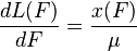
- If the Lorenz curve is twice differentiable, then the probability density function f(x) exists at that point and:
- If L(F) is continuously differentiable, then the tangent of L(F) is parallel to the line of perfect equality at the point F(μ). This is also the point at which the equality gap F − L(F), the vertical distance between the Lorenz curve and the line of perfect equality, is greatest. The size of the gap is equal to half of the relative mean deviation:

[edit] See also
- Distribution (economics)
- Distribution of wealth
- Welfare economics
- Income inequality metrics
- Gini coefficient
- Robin Hood index
- ROC analysis
- Social welfare (political science)
- Economic inequality
- Zipf's law
- Pareto distribution
- mean deviation
[edit] References
- ^ Sullivan, arthur; Steven M. Sheffrin (2003). Economics: Principles in action. Upper Saddle River, New Jersey 07458: Pearson Prentice Hall. pp. 349. ISBN 0-13-063085-3. http://www.pearsonschool.com/index.cfm?locator=PSZ3R9&PMDbSiteId=2781&PMDbSolutionId=6724&PMDbCategoryId=&PMDbProgramId=12881&level=4.
[edit] Citations
- Lorenz, M. O. (1905). "Methods of measuring the concentration of wealth". Publications of the American Statistical Association 9: 209–219. doi:.
- Gastwirth, Joseph L. (1972). "The Estimation of the Lorenz Curve and Gini Index". The Review of Economics and Statistics 54: 306–316. doi:.
- Chakravarty, S. R. (1990). Ethical Social Index Numbers. New York: Springer-Verlag.
- Anand, Sudhir (1983). Inequality and Poverty in Malaysia. New York: Oxford University Press.
[also Will Dawson's contributions]
[edit] External links
- Measuring income inequality: a new database, with link to dataset
- Free Online Software (Calculator) computes the Gini Coefficient, plots the Lorenz curve, and computes many other measures of concentration for any dataset
- Free Calculator: Online and downloadable scripts (Python and Lua) for Atkinson, Gini, and Hoover inequalities
- Users of the R data analysis software can install the "ineq" package which allows for computation of a variety of inequality indices including Gini, Atkinson, Theil.
- A MATLAB Inequality Package, including code for computing Gini, Atkinson, Theil indexes and for plotting the Lorenz Curve. Many examples are available.

