State space (controls)

From Wikipedia, the free encyclopedia

In control engineering, a state space representation is a mathematical model of a physical system as a set of input, output and state variables related by first-order differential equations. To abstract from the number of inputs, outputs and states, the variables are expressed as vectors and the differential and algebraic equations are written in matrix form (the last one can be done when the dynamical system is linear and time invariant). The state space representation (also known as the "time-domain approach") provides a convenient and compact way to model and analyze systems with multiple inputs and outputs. With $p$ inputs and $q$ outputs, we would otherwise have to write down $q \times p$ Laplace transforms to encode all the information about a system. Unlike the frequency domain approach, the use of the state space representation is not limited to systems with linear components and zero initial conditions. "State space" refers to the space whose axes are the state variables. The state of the system can be represented as a vector within that space.

[edit] State variables

Typical state space model

The internal state variables are the smallest possible subset of system variables that can represent the entire state of the system at any given time. State variables must be linearly independent; a state variable cannot be a linear combination of other state variables. The minimum number of state variables required to represent a given system, $n$ , is usually equal to the order of the system's defining differential equation. If the system is represented in transfer function form, the minimum number of state variables is equal to the order of the transfer function's denominator after it has been reduced to a proper fraction. It is important to understand that converting a state space realization to a transfer function form may lose some internal information about the system, and may provide a description of a system which is stable, when the state-space realization is unstable at certain points. In electric circuits, the number of state variables is often, though not always, the same as the number of energy storage elements in the circuit such as capacitors and inductors.

[edit] Linear systems

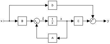
The most general state space representation of a linear system with $p$ inputs, $q$ outputs and $n$ state variables is written in the following form:

$\dot{\mathbf{x}}(t) = A(t) \mathbf{x}(t) + B(t) \mathbf{u}(t)$

$\mathbf{y}(t) = C(t) \mathbf{x}(t) + D(t) \mathbf{u}(t)$

where:

$x(\cdot)$ is called the "state vector" - $x(t) \in \mathbb{R}^n$ ;

$y(\cdot)$ is called the "output vector" - $y(t) \in \mathbb{R}^q$ ;

$u(\cdot)$ is called the "input (or control) vector" - $u(t) \in \mathbb{R}^p$ ;

$A(\cdot)$ is the "state matrix" - $\operatorname{dim}[A(\cdot)] = n \times n$ ,

$B(\cdot)$ is the "input matrix" - $\operatorname{dim}[B(\cdot)] = n \times p$ ,

$C(\cdot)$ is the "output matrix" - $\operatorname{dim}[C(\cdot)] = q \times n$ ,

$D(\cdot)$ is the "feedthrough (or feedforward) matrix" - $\operatorname{dim}[D(\cdot)] = q \times p$ ,

$\dot{\mathbf{x}}(t) := {d\mathbf{x}(t) \over dt}$ .

For simplicity, $D(\cdot)$ is often chosen to be the zero matrix, i.e. the system is chosen not to have direct feedthrough. Notice that in this general formulation, all matrices are supposed to be time-variant, i.e. some or all their elements can depend on time. The time variable $t$ can be a "continuous" one (i.e. $t \in \mathbb{R}$ ) or a discrete one (i.e. $t \in \mathbb{Z}$ ): in the latter case the time variable is usually indicated as $k$ . Depending on the assumptions taken, the state-space model representation can assume the following forms:

System type	State-space model
Continuous time-invariant	$\dot{\mathbf{x}}(t) = A \mathbf{x}(t) + B \mathbf{u}(t)$ $\mathbf{y}(t) = C \mathbf{x}(t) + D \mathbf{u}(t)$
Continuous time-variant	$\dot{\mathbf{x}}(t) = \mathbf{A}(t) \mathbf{x}(t) + \mathbf{B}(t) \mathbf{u}(t)$ $\mathbf{y}(t) = \mathbf{C}(t) \mathbf{x}(t) + \mathbf{D}(t) \mathbf{u}(t)$
Discrete time-invariant	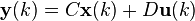$\mathbf{x}(k+1) = A \mathbf{x}(k) + B \mathbf{u}(k)$ $\mathbf{y}(k) = C \mathbf{x}(k) + D \mathbf{u}(k)$
Discrete time-variant	$\mathbf{x}(k+1) = \mathbf{A}(k) \mathbf{x}(k) + \mathbf{B}(k) \mathbf{u}(k)$ $\mathbf{y}(k) = \mathbf{C}(k) \mathbf{x}(k) + \mathbf{D}(k) \mathbf{u}(k)$
Laplace domain of continuous time-invariant	$s \mathbf{X}(s) = A \mathbf{X}(s) + B \mathbf{U}(s)$ $\mathbf{Y}(s) = C \mathbf{X}(s) + D \mathbf{U}(s)$
Z-domain of discrete time-invariant	$z \mathbf{X}(z) = A \mathbf{X}(z) + B \mathbf{U}(z)$ $\mathbf{Y}(z) = C \mathbf{X}(z) + D \mathbf{U}(z)$

Stability and natural response characteristics of a system can be studied from the eigenvalues of the matrix A. The stability of a time-invariant state-space model can easily be determined by looking at the system's transfer function in factored form. It will then look something like this:

$\textbf{G}(s) = k \frac{ (s - z_{1})(s - z_{2})(s - z_{3}) }{ (s - p_{1})(s - p_{2})(s - p_{3})(s - p_{4}) }$

The denominator of the transfer function is equal to the characteristic polynomial found by taking the determinant of $s I - A$ ,

$\mathbf{\lambda}(s) = |sI - A|$ .

The roots of this polynomial (the eigenvalues) yield the poles in the system's transfer function. These poles can be used to analyze whether the system is asymptotically stable or marginally stable. An alternative approach to determining stability, which does not involve calculating eigenvalues, is to analyze the system's Lyapunov stability. The zeros found in the numerator of $\textbf{G}(s)$ can similarly be used to determine whether the system is minimum phase.

The system may still be input–output stable (see BIBO stable) even though it is not internally stable. This may be the case if unstable poles are canceled out by zeros.

[edit] Controllability

Main article: Controllability

Thus state controllability condition implies that it is possible - by admissible inputs - to steer the states from any initial value to any final value within some time window. A continuous time-invariant state-space model is controllable if and only if

$\operatorname{rank}\begin{bmatrix}B& AB& A^{2}B& ...& A^{n-1}B\end{bmatrix} = n$

[edit] Observability

Main article: Observability

Observability is a measure for how well internal states of a system can be inferred by knowledge of its external outputs. The observability and controllability of a system are mathematical duals.

A continuous time-invariant state-space model is observable if and only if

$\operatorname{rank}\begin{bmatrix}C\\ CA\\ ...\\ CA^{n-1}\end{bmatrix} = n$

(Rank is the number of linearly independent rows in a matrix.)

[edit] Transfer function

The "transfer function" of a continuous time-invariant state-space model can be derived in the following way:

First, taking the laplace transform of

$\dot{\mathbf{x}}(t) = A \mathbf{x}(t) + B \mathbf{u}(t)$

yields

$s\mathbf{X}(s) = A \mathbf{X}(s) + B \mathbf{U}(s)$

Next, we simplify for $\mathbf{X}(s)$ , giving

$(s\mathbf{I} - A)\mathbf{X}(s) = B\mathbf{U}(s)$

$\mathbf{X}(s) = (s\mathbf{I} - A)^{-1}B\mathbf{U}(s)$

this is substituted for $\mathbf{X}(s)$ in the output equation

$\mathbf{Y}(s) = C\mathbf{X}(s) + D\mathbf{U}(s)$ , giving

$\mathbf{Y}(s) = C((s\mathbf{I} - A)^{-1}B\mathbf{U}(s)) + D\mathbf{U}(s)$

Since the transfer function $\mathbf{G}(s)$ is defined as the ratio of the output to the input of a system, we take

$\mathbf{G}(s) = \mathbf{Y}(s) / \mathbf{U}(s)$

and substitute the previous expression for $\mathbf{Y}(s)$ with respect to $\mathbf{U}(s)$ , giving

$\mathbf{G}(s) = C(s\mathbf{I} - A)^{-1}B + D$

Clearly $\mathbf{G}(s)$ must have $q$ by $p$ dimensionality, and thus has a total of $q p$ elements. So for every input there are $q$ transfer functions with one for each output. This is why the state-space representation can easily be the preferred choice for multiple-input, multiple-output (MIMO) systems.

[edit] Canonical realizations

Any given transfer function which is strictly proper can easily be transferred into state-space by the following approach (this example is for a 4-dimensional, single-input, single-output system)):

Given a transfer function, expand it to reveal all coefficients in both the numerator and denominator. This should result in the following form:

$\textbf{G}(s) = \frac{n_{1}s^{3} + n_{2}s^{2} + n_{3}s + n_{4}}{s^{4} + d_{1}s^{3} + d_{2}s^{2} + d_{3}s + d_{4}}$ .

The coefficients can now be inserted directly into the state-space model by the following approach:

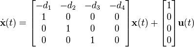
$\dot{\textbf{x}}(t) = \begin{bmatrix} -d_{1}& -d_{2}& -d_{3}& -d_{4}\\ 1& 0& 0& 0\\ 0& 1& 0& 0\\ 0& 0& 1& 0 \end{bmatrix}\textbf{x}(t) + \begin{bmatrix} 1\\ 0\\ 0\\ 0\\ \end{bmatrix}\textbf{u}(t)$

$\textbf{y}(t) = \begin{bmatrix} n_{1}& n_{2}& n_{3}& n_{4} \end{bmatrix}\textbf{x}(t)$ .

This state-space realization is called controllable canonical form because the resulting model is guaranteed to be controllable.

The transfer function coefficients can also be used to construct another type of canonical form

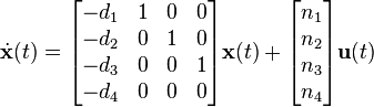
$\dot{\textbf{x}}(t) = \begin{bmatrix} -d_{1}& 1& 0& 0\\ -d_{2}& 0& 1& 0\\ -d_{3}& 0& 0& 1\\ -d_{4}& 0& 0& 0 \end{bmatrix}\textbf{x}(t) + \begin{bmatrix} n_{1}\\ n_{2}\\ n_{3}\\ n_{4} \end{bmatrix}\textbf{u}(t)$

$\textbf{y}(t) = \begin{bmatrix} 1& 0& 0& 0 \end{bmatrix}\textbf{x}(t)$ .

This state-space realization is called observable canonical form because the resulting model is guaranteed to be observable.

[edit] Proper transfer functions

Transfer functions which are only proper (and not strictly proper) can also be realised quite easily. The trick here is to separate the transfer function into two parts: a strictly proper part and a constant.

$\textbf{G}(s) = \textbf{G}_{SP}(s) + \textbf{G}(\infty)$

The strictly proper transfer function can then be transformed into a canonical state space realization using techniques shown above. The state space realization of the constant is trivially $\textbf{y}(t) = \textbf{G}(\infty)\textbf{u}(t)$ . Together we then get a state space realization with matrices A,B and C determined by the strictly proper part, and matrix D determined by the constant.

Here is an example to clear things up a bit:

$\textbf{G}(s) = \frac{s^{2} + 3s + 3}{s^{2} + 2s + 1} = \frac{s + 2}{s^{2} + 2s + 1} + 1$

which yields the following controllable realization

$\dot{\textbf{x}}(t) = \begin{bmatrix} -2& -1\\ 1& 0\\ \end{bmatrix}\textbf{x}(t) + \begin{bmatrix} 1\\ 0\end{bmatrix}\textbf{u}(t)$

$\textbf{y}(t) = \begin{bmatrix} 1& 2\end{bmatrix}\textbf{x}(t) + \begin{bmatrix} 1\end{bmatrix}\textbf{u}(t)$

Notice how the output also depends directly on the input. This is due to the $\textbf{G}(\infty)$ constant in the transfer function.

[edit] Feedback

Typical state space model with feedback

A common method for feedback is to multiply the output by a matrix K and setting this as the input to the system: $\mathbf{u}(t) = K \mathbf{y}(t)$ . Since the values of K are unrestricted the values can easily be negated for negative feedback. The presence of a negative sign (the common notation) is merely a notational one and its absence has no impact on the end results.

$\dot{\mathbf{x}}(t) = A \mathbf{x}(t) + B \mathbf{u}(t)$

$\mathbf{y}(t) = C \mathbf{x}(t) + D \mathbf{u}(t)$

becomes

$\dot{\mathbf{x}}(t) = A \mathbf{x}(t) + B K \mathbf{y}(t)$

$\mathbf{y}(t) = C \mathbf{x}(t) + D K \mathbf{y}(t)$

solving the output equation for $\mathbf{y}(t)$ and substituting in the state equation results in

$\dot{\mathbf{x}}(t) = \left(A + B K \left(I - D K\right)^{-1} C \right) \mathbf{x}(t)$

$\mathbf{y}(t) = \left(I - D K\right)^{-1} C \mathbf{x}(t)$

The advantage of this is that the eigenvalues of A can be controlled by setting K appropriately through eigendecomposition of $\left(A + B K \left(I - D K\right)^{-1} C \right)$ . This assumes that the open-loop system is controllable or that the unstable eigenvalues of A can be made stable through appropriate choice of K.

One fairly common simplification to this system is removing D and setting C to identity, which reduces the equations to

$\dot{\mathbf{x}}(t) = \left(A + B K \right) \mathbf{x}(t)$

$\mathbf{y}(t) = \mathbf{x}(t)$

This reduces the necessary eigendecomposition to just $A + B K$ .

[edit] Feedback with setpoint (reference) input

Output feedback with set point

In addition to feedback, an input, $r (t)$ , can be added such that $\mathbf{u}(t) = -K \mathbf{y}(t) + \mathbf{r}(t)$ .

$\dot{\mathbf{x}}(t) = A \mathbf{x}(t) + B \mathbf{u}(t)$

$\mathbf{y}(t) = C \mathbf{x}(t) + D \mathbf{u}(t)$

becomes

$\dot{\mathbf{x}}(t) = A \mathbf{x}(t) - B K \mathbf{y}(t) + B \mathbf{r}(t)$

$\mathbf{y}(t) = C \mathbf{x}(t) - D K \mathbf{y}(t) + D \mathbf{r}(t)$

solving the output equation for $\mathbf{y}(t)$ and substituting in the state equation results in

$\dot{\mathbf{x}}(t) = \left(A - B K \left(I + D K\right)^{-1} C \right) \mathbf{x}(t) + B \left(I - K \left(I + D K\right)^{-1}D \right) \mathbf{r}(t)$

$\mathbf{y}(t) = \left(I + D K\right)^{-1} C \mathbf{x}(t) + \left(I + D K\right)^{-1} D \mathbf{r}(t)$

One fairly common simplification to this system is removing D, which reduces the equations to

$\dot{\mathbf{x}}(t) = \left(A - B K C \right) \mathbf{x}(t) + B \mathbf{r}(t)$

$\mathbf{y}(t) = C \mathbf{x}(t)$

[edit] Moving object example

A classical linear system is that of one-dimensional movement of an object. The Newton's laws of motion for an object moving horizontally on a plane and attached to a wall with a spring

$m \ddot{y}(t) = u(t) - k_1 \dot{y}(t) - k_2 y(t)$

where

$y (t)$ is position; $\dot y(t)$ is velocity; $\ddot{y}(t)$ is acceleration
$u (t)$ is an applied force
$k 1$ is the viscous friction coefficient
$k 2$ is the spring constant
$m$ is the mass of the object

The state equation would then become

$\left[ \begin{matrix} \mathbf{\dot{x_1}}(t) \\ \mathbf{\dot{x_2}}(t) \end{matrix} \right] = \left[ \begin{matrix} 0 & 1 \\ -\frac{k_2}{m} & -\frac{k_1}{m} \end{matrix} \right] \left[ \begin{matrix} \mathbf{x_1}(t) \\ \mathbf{x_2}(t) \end{matrix} \right] + \left[ \begin{matrix} 0 \\ \frac{1}{m} \end{matrix} \right] \mathbf{u}(t)$

$\mathbf{y}(t) = \left[ \begin{matrix} 1 & 0 \end{matrix} \right] \left[ \begin{matrix} \mathbf{x_1}(t) \\ \mathbf{x_2}(t) \end{matrix} \right]$

where

$x 1 (t)$ represents the position of the object
$x_2(t) = \dot{x_1}(t)$ is the velocity of the object
$\dot{x_2}(t) = \ddot{x_1}(t)$ is the acceleration of the object
the output $\mathbf{y}(t)$ is the position of the object

The controllability test is then

$\left[ \begin{matrix} B & AB \end{matrix} \right] = \left[ \begin{matrix} \left[ \begin{matrix} 0 \\ \frac{1}{m} \end{matrix} \right] & \left[ \begin{matrix} 0 & 1 \\ -\frac{k_2}{m} & -\frac{k_1}{m} \end{matrix} \right] \left[ \begin{matrix} 0 \\ \frac{1}{m} \end{matrix} \right] \end{matrix} \right] = \left[ \begin{matrix} 0 & \frac{1}{m} \\ \frac{1}{m} & \frac{k_1}{m^2} \end{matrix} \right]$

which has full rank for all $k 1$ and $m$ .

The observability test is then

$\left[ \begin{matrix} C \\ CA \end{matrix} \right] = \left[ \begin{matrix} \left[ \begin{matrix} 1 & 0 \end{matrix} \right] \\ \left[ \begin{matrix} 1 & 0 \end{matrix} \right] \left[ \begin{matrix} 0 & 1 \\ -\frac{k_2}{m} & -\frac{k_1}{m} \end{matrix} \right] \end{matrix} \right] = \left[ \begin{matrix} 1 & 0 \\ 0 & 1 \end{matrix} \right]$

which also has full rank. Therefore, this system is both controllable and observable.

[edit] Nonlinear systems

The more general form of a state space model can be written as two functions.

$\mathbf{\dot{x}}(t) = \mathbf{f}(t, x(t), u(t))$

$\mathbf{y}(t) = \mathbf{h}(t, x(t), u(t))$

The first is the state equation and the latter is the output equation. If the function $f(\cdot,\cdot,\cdot)$ is a linear combination of states and inputs then the equations can be written in matrix notation like above. The $u (t)$ argument to the functions can be dropped if the system is unforced (i.e., it has no inputs).

[edit] Pendulum example

A classic nonlinear system is a simple unforced pendulum

$ml\ddot\theta(t)= -mg\sin\theta(t) - kl\dot\theta(t)$

where

$θ(t)$ is the angle of the pendulum with respect to the direction of gravity
$m$ is the mass of the pendulum (pendulum rod's mass is assumed to be zero)
$g$ is the gravitational acceleration
$k$ is coefficient of friction at the pivot point
$l$ is the radius of the pendulum (to the center of gravity of the mass $m$ )

The state equations are then

$\dot{x_1}(t) = x_2(t)$

$\dot{x_2}(t) = - \frac{g}{l}\sin{x_1}(t) - \frac{k}{m}{x_2}(t)$

where

$x 1 (t): = θ(t)$ is the angle of the pendulum
$x_2(t) :=\dot{x_1}(t)$ is the rotational velocity of the pendulum
$\dot{x_2} =\ddot{x_1}$ is the rotational acceleration of the pendulum

Instead, the state equation can be written in the general form

$\dot{x}(t) = \left( \begin{matrix} \dot{x_1}(t) \\ \dot{x_2}(t) \end{matrix} \right) = \mathbf{f}(t, x(t)) = \left( \begin{matrix} x_2(t) \\ - \frac{g}{l}\sin{x_1}(t) - \frac{k}{m}{x_2}(t) \end{matrix} \right).$

The equilibrium/stationary points of a system are when $\dot{x} = 0$ and so the equilibrium points of a pendulum are those that satisfy

$\left( \begin{matrix} x_1 \\ x_2 \end{matrix} \right) = \left( \begin{matrix} n\pi \\ 0 \end{matrix} \right)$

for integers n.

[edit] References

Chen, Chi-Tsong 1999. Linear System Theory and Design, 3rd. ed., Oxford University Press (ISBN 0-19-511777-8)
Khalil, Hassan K. Nonlinear Systems, 3rd. ed., Prentice Hall (ISBN 0-13-067389-7)
Nise, Norman S. 2004. Control Systems Engineering, 4th ed., John Wiley & Sons, Inc. (ISBN 0-471-44577-0)
Hinrichsen, Diederich and Pritchard, Anthony J. 2005. Mathematical Systems Theory I, Modelling, State Space Analysis, Stability and Robustness. Springer. (ISBN 978-3-540-44125-0)
Sontag, Eduardo D. 1999. Mathematical Control Theory: Deterministic Finite Dimensional Systems. Second Edition. Springer. (ISBN 0-387-984895) (available free online)
Friedland, Bernard. 2005. Control System Design: An Introduction to State Space Methods. Dover. (ISBN 0486442780).

On the applications of state space models in econometrics:

Durbin, J. and S. Koopman (2001). Time series analysis by state space methods. Oxford University Press, Oxford.

[edit] See also

Control engineering
Control theory
State observer
Discretization of state space models
Phase space for information about phase state (like state space) in physics and mathematics.
State space for information about state space with discrete states in computer science.
State space (physics) for information about state space in physics.

State space (controls)

From Wikipedia, the free encyclopedia

Contents

[edit] State variables

[edit] Linear systems

[edit] Controllability

[edit] Observability

[edit] Transfer function

[edit] Canonical realizations

[edit] Proper transfer functions

[edit] Feedback

[edit] Feedback with setpoint (reference) input

[edit] Moving object example

[edit] Nonlinear systems

[edit] Pendulum example

[edit] References

[edit] See also

Views

Personal tools

Navigation

Search

Interaction

Toolbox

Languages