Expected value

From Wikipedia, the free encyclopedia

"Expectation value" redirects here. For the expectation value in quantum mechanics, see expectation value (quantum mechanics).

In probability theory and statistics, the expected value (or expectation value, or mathematical expectation, or mean, or first moment) of a random variable is the integral of the random variable with respect to its probability measure. For discrete random variables this is equivalent to the probability-weighted sum of the possible values, and for continuous random variables with a density function it is the probability density -weighted integral of the possible values.

The term "expected value" can be misleading. It must not be confused with the "most probable value." The expected value is in general not a typical value that the random variable can take on. It is often helpful to interpret the expected value of a random variable as the long-run average value of the variable over many independent repetitions of an experiment.

The expected value may be intuitively understood by the law of large numbers: The expected value, when it exists, is almost surely the limit of the sample mean as sample size grows to infinity. The value may not be expected in the general sense – the "expected value" itself may be unlikely or even impossible (such as having 2.5 children), just like the sample mean. The expected value does not exist for all distributions, such as the Cauchy distribution.

It is possible to construct an expected value equal to the probability of an event by taking the expectation of an indicator function that is one if the event has occurred and zero otherwise. This relationship can be used to translate properties of expected values into properties of probabilities, e.g. using the law of large numbers to justify estimating probabilities by frequencies.

[edit] Examples

The expected value from the roll of an ordinary six-sided die is

$\operatorname{E}({\rm Roll\ With\ 6\ Sided\ Die}) = \frac{1 + 2 + 3 + 4 + 5 + 6}{6} = 3.5$

which is not among the possible outcomes.

A common application of expected value is gambling. For example, an American roulette wheel has 38 places where the ball may land, all equally likely. A winning bet on a single number pays 35-to-1, meaning that the original stake is not lost, and 35 times that amount is won, so you receive 36 times what you've bet. Considering all 38 possible outcomes, the expected value of the profit resulting from a dollar bet on a single number is the sum of what you may lose times the odds of losing and what you will win times the odds of winning, that is,

$\operatorname{E}({\rm winnings\ \$1\ bet}) = \left( -$1 \times \frac{37}{38} \right) + \left( $35 \times \frac{1}{38} \right) = -$\frac{1}{19} \approx -$0.0526.$

The change in your financial holdings is −$1 when you lose, and $35 when you win. Thus one may expect, on average, to lose about five cents for every dollar bet, and the expected value of a one-dollar bet is $0.9474. In gambling, an event of which the expected value equals the stake (of which the bettor's expected profit is zero) is called a "fair game."

[edit] Mathematical definition

In general, if $X\,$ is a random variable defined on a probability space $(\Omega, \Sigma, P)\,$ , then the expected value of $X\,$ , denoted $\operatorname{E}(X)\,$ , $\langle X \rangle$ , $\bar{X}$ or $\mathbb{E}(X)$ , is defined as

$\operatorname{E}(X) = \int_\Omega X\, \operatorname{d}P$

where the Lebesgue integral is employed. Note that not all random variables have an expected value, since the integral may not exist (e.g., Cauchy distribution). Two variables with the same probability distribution will have the same expected value, if it is defined.

If $X$ is a discrete random variable with probability mass function $p (x)$ , then the expected value becomes

$\operatorname{E}(X) = \sum_i x_i p(x_i) \,$

as in the gambling example mentioned above.

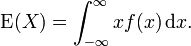
If the probability distribution of $X$ admits a probability density function $f (x)$ , then the expected value can be computed as

$\operatorname{E}(X) = \int_{-\infty}^\infty x f(x)\, \operatorname{d}x .$

It follows directly from the discrete case definition that if $X$ is a constant random variable, i.e. $X = b$ for some fixed real number $b$ , then the expected value of $X$ is also $b$ .

The expected value of an arbitrary function of X, g(X), with respect to the probability density function f(x) is given by the inner product of f and g:

$\operatorname{E}(g(X)) = \int_{-\infty}^\infty g(x) f(x)\, \operatorname{d}x .$

Using representations as Riemann–Stieltjes integral and integration by parts the formula can be restated as

$\operatorname{E}(g(X)) = \int_a^\infty g(x) \, d \operatorname{P}(X \le x)= g(a)+ \int_a^\infty g'(x)\operatorname{P}(X > x) \, d x$

if $\operatorname{P}(X \ge a)=1$ .

As a special case let $α$ denote a positive real number, then

$\operatorname{E}(\left|X \right|^\alpha) = \alpha \int_{0}^{\infty} t^{\alpha -1}\operatorname{P}(\left|X \right|>t) \, \operatorname{d}t.$

In particular, for $α = 1$ , this reduces to:

$\operatorname{E}(X) = \int_{0}^{\infty} \lbrace 1-F(t) \rbrace \, \operatorname{d}t,$

if $P[X \ge 0]=1$ .

[edit] Conventional terminology

When one speaks of the "expected price", "expected height", etc. one means the expected value of a random variable that is a price, a height, etc.
When one speaks of the "expected number of attempts needed to get one successful attempt," one might conservatively approximate it as the reciprocal of the probability of success for such an attempt. Cf. expected value of the geometric distribution.

[edit] Properties

[edit] Constants

The expected value of a constant is equal to the constant itself; i.e., if 'c' is a constant, then $\operatorname{E}(c) = c$ .

[edit] Monotonicity

If X and Y are random variables so that $X \le Y$ almost surely, then $\operatorname{E}(X) \le \operatorname{E}(Y)$ .

[edit] Linearity

The expected value operator (or expectation operator) $\operatorname{E}$ is linear in the sense that

$\operatorname{E}(X + c)= \operatorname{E}(X) + c\,$

$\operatorname{E}(X + Y)= \operatorname{E}(X) + \operatorname{E}(Y)\,$

$\operatorname{E}(aX)= a \operatorname{E}(X)\,$

Note that the second result is valid even if X is not statistically independent of Y. Combining the results from previous three equations, we can see that

$\operatorname{E}(aX + b)= a \operatorname{E}(X) + b\,$

$\operatorname{E}(a X + b Y) = a \operatorname{E}(X) + b \operatorname{E}(Y)\,$

for any two random variables $X$ and $Y$ (which need to be defined on the same probability space) and any real numbers $a$ and $b$ .

[edit] Iterated expectation

[edit] Iterated expectation for discrete random variables

For any two discrete random variables $X, Y$ one may define the conditional expectation:

$\operatorname{E}(X|Y)(y) = \operatorname{E}(X|Y=y) = \sum\limits_x x \cdot \operatorname{P}(X=x|Y=y).$

which means that $\operatorname{E}(X|Y)(y)$ is a function on $y$ .

Then the expectation of $X$ satisfies

$\operatorname{E} \left( \operatorname{E}(X|Y) \right)= \sum\limits_y \operatorname{E}(X|Y=y) \cdot \operatorname{P}(Y=y) \,$

$=\sum\limits_y \left( \sum\limits_x x \cdot \operatorname{P}(X=x|Y=y) \right) \cdot \operatorname{P}(Y=y)\,$

$=\sum\limits_y \sum\limits_x x \cdot \operatorname{P}(X=x|Y=y) \cdot \operatorname{P}(Y=y)\,$

$=\sum\limits_y \sum\limits_x x \cdot \operatorname{P}(Y=y|X=x) \cdot \operatorname{P}(X=x) \,$

$=\sum\limits_x x \cdot \operatorname{P}(X=x) \cdot \left( \sum\limits_y \operatorname{P}(Y=y|X=x) \right) \,$

$=\sum\limits_x x \cdot \operatorname{P}(X=x) \,$

$=\operatorname{E}(X).\,$

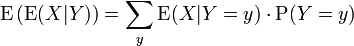
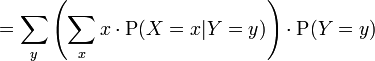
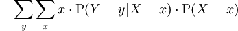
Hence, the following equation holds:

$\operatorname{E}(X) = \operatorname{E} \left( \operatorname{E}(X|Y) \right).$

The right hand side of this equation is referred to as the iterated expectation and is also sometimes called the tower rule. This proposition is treated in law of total expectation.

[edit] Iterated expectation for continuous random variables

In the continuous case, the results are completely analogous. The definition of conditional expectation would use inequalities, density functions, and integrals to replace equalities, mass functions, and summations, respectively. However, the main result still holds:

$\operatorname{E}(X) = \operatorname{E} \left( \operatorname{E}(X|Y) \right).$

[edit] Inequality

If a random variable X is always less than or equal to another random variable Y, the expectation of X is less than or equal to that of Y:

If $X \leq Y$ , then $\operatorname{E}(X) \leq \operatorname{E}(Y)$ .

In particular, since $X \leq |X|$ and $-X \leq |X|$ , the absolute value of expectation of a random variable is less than or equal to the expectation of its absolute value:

$|\operatorname{E}(X)| \leq \operatorname{E}(|X|)$

[edit] Non-multiplicativity

In general, the expected value operator is not multiplicative, i.e. $\operatorname{E}(X Y)$ is not necessarily equal to $\operatorname{E}(X) \operatorname{E}(Y)$ . If multiplicativity occurs, the $X$ and $Y$ variables are said to be uncorrelated (independent variables are a notable case of uncorrelated variables). The lack of multiplicativity gives rise to study of covariance and correlation.

If one considers the joint PDF of X and Y, say j(X,Y), then the expectation of XY is

$E(XY)=\int_{X,Y}XYj(X,Y)\,dX\,dY.$

Now if X and Y are independent, then by definition j(X,Y)=f(X)g(Y) where f and g are the marginal PDFs for X and Y. Then

$E(XY)=\int_{X,Y}XYf(X)g(Y)\,dX\,dY= \int_X\int_Y XYf(X)g(Y)\,dX\,dY= \int_X Xf(X)\left[\int Yg(Y)\,dY\right]\,dX=\int_XXf(X)E(Y)\,dX=E(X)E(Y)$

Observe that independence of X and Y is required only to write j(X,Y)=f(X)g(Y), and this is required to establish the third equality above.

[edit] Functional non-invariance

In general, the expectation operator and functions of random variables do not commute; that is

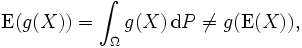
$\operatorname{E}(g(X)) = \int_{\Omega} g(X)\, \operatorname{d}P \neq g(\operatorname{E}(X)),$

A notable inequality concerning this topic is Jensen's inequality, involving expected values of convex (or concave) functions.

[edit] The law of the unconscious statistician

Main article: Law of the unconscious statistician

[edit] Uses and applications of the expected value

The expected values of the powers of $X$ are called the moments of $X$ ; the moments about the mean of $X$ are expected values of powers of $X - \operatorname{E}(X)$ . The moments of some random variables can be used to specify their distributions, via their moment generating functions.

To empirically estimate the expected value of a random variable, one repeatedly measures observations of the variable and computes the arithmetic mean of the results. If the expected value exists, this procedure estimates the true expected value in an unbiased manner and has the property of minimizing the sum of the squares of the residuals (the sum of the squared differences between the observations and the estimate). The law of large numbers demonstrates (under fairly mild conditions) that, as the size of the sample gets larger, the variance of this estimate gets smaller.

In classical mechanics, the center of mass is an analogous concept to expectation. For example, suppose $X$ is a discrete random variable with values $x i$ and corresponding probabilities $p i$ . Now consider a weightless rod on which are placed weights, at locations $x i$ along the rod and having masses $p i$ (whose sum is one). The point at which the rod balances is $\operatorname{E}(X)$ .

Expected values can also be used to compute the variance, by means of the computational formula for the variance

$\operatorname{Var}(X)= \operatorname{E}(X^2) - (\operatorname{E}(X))^2.$

A very important application of the expectation value is in the field of quantum mechanics. The expectation value of a quantum mechanical operator $\hat{A}$ operating on a quantum state vector $|\psi\rangle$ is written as $\langle\hat{A}\rangle = \langle\psi|A|\psi\rangle$ . The uncertainty in $\hat{A}$ can be calculated using the formula $(\Delta A)^2 = \langle\hat{A}^2\rangle - \langle\hat{A}\rangle^2$ .

[edit] Expectation of matrices

If $X$ is an $m \times n$ matrix, then the expected value of the matrix is defined as the matrix of expected values:

$\operatorname{E}(X) = \operatorname{E} \begin{pmatrix} x_{1,1} & x_{1,2} & \cdots & x_{1,n} \\ x_{2,1} & x_{2,2} & \cdots & x_{2,n} \\ \vdots & \vdots & \ddots & \vdots \\ x_{m,1} & x_{m,2} & \cdots & x_{m,n} \end{pmatrix} = \begin{pmatrix} \operatorname{E}(x_{1,1}) & \operatorname{E}(x_{1,2}) & \cdots & \operatorname{E}(x_{1,n}) \\ \operatorname{E}(x_{2,1}) & \operatorname{E}(x_{2,2}) & \cdots & \operatorname{E}(x_{2,n}) \\ \vdots & \vdots & \ddots & \vdots \\ \operatorname{E}(x_{m,1}) & \operatorname{E}(x_{m,2}) & \cdots & \operatorname{E}(x_{m,n}) \end{pmatrix}.$

This is utilized in covariance matrices.

[edit] Computation

It is often useful to update a computed expected value as new data come in. This can be done as follows, where $n e w_v a l u e$ is the $c o u n t$ -th value, and we use the previous estimate $\operatorname{E}_\mathrm{prev}(X)$ to compute $\operatorname{E}_\mathrm{new}(X)$ :

$\operatorname{E}_\mathrm{new}(X) = \frac{(\text{count}-1) \cdot \operatorname{E}_\mathrm{prev}(X) + (\text{new value})}{\text{count}}$

[edit] Formulas for special cases

[edit] Discrete distribution taking only non-negative integer values

When a random variable takes only values in ${0,1,2,3,...}$ we can use the following formula for computing its expectation:

$\operatorname{E}(X)=\sum\limits_{i=1}^\infty P(X\geq i).$

Proof:

$\begin{align} \sum\limits_{i=1}^\infty P(X\geq i)&=\sum\limits_{i=1}^\infty \sum\limits_{j=i}^\infty P(X = j) \end{align}$

interchanging the order of summation, we have

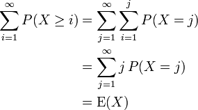
$\begin{align} \sum\limits_{i=1}^\infty P(X\geq i)&=\sum\limits_{j=1}^\infty \sum\limits_{i=1}^j P(X = j)\\ &=\sum\limits_{j=1}^\infty j\, P(X = j)\\ &=\operatorname{E}(X) \end{align}$

as claimed. This result can be a useful computational shortcut. For example, suppose we toss a coin where the probability of heads is $p$ . How many tosses can we expect until the first heads? Let $X$ be this number. Note that we are counting only the tails and not the heads which ends the experiment; in particular, we can have $X = 0$ . The expectation of $X$ may be computed by $\sum_{i= 1}^\infty (1-p)^i=\frac{1-p}{p}$ . This is because the number of tosses is at least $i$ exactly when the first $i$ tosses yielded tails. This matches the expectation of a random variable with an Exponential distribution. We used the formula for Geometric progression: $\sum_{k=1}^\infty r^k=\frac{r}{1-r}.$

[edit] Continuous distribution taking non-negative values

Analogously with the discrete case above, when a continuous random variable X takes only non-negative values, we can use the following formula for computing its expectation:

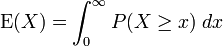
$\operatorname{E}(X)=\int_0^\infty P(X \ge x)\; dx$

Proof:

$\begin{align} \int_0^\infty P(X\ge x)\;dx &=\int_0^\infty \int_x^\infty f_X(t)\;dt\;dx \end{align}$

interchanging the order of integration, we have

$\begin{align} \int_0^\infty P(X\ge x)\;dx &= \int_0^\infty \int_0^t f_X(t)\;dx\;dt \\ &= \int_0^\infty t f_X(t)\;dt\\ &=\operatorname{E}(X) \end{align}$

as claimed.

[edit] See also

Conditional expectation
An inequality on location and scale parameters
Expected value is also a key concept in economics, finance, and bioinformatics.
The general term expectation
Pascal's Wager
Moment (mathematics)
Expectation value (quantum mechanics)
St. Petersburg Paradox
Buffon's noodle

[edit] External links

Expectation on PlanetMath