Expectation-maximization algorithm

From Wikipedia, the free encyclopedia

An expectation-maximization (EM) algorithm is used in statistics for finding maximum likelihood estimates of parameters in probabilistic models, where the model depends on unobserved latent variables. EM is an iterative method which alternates between performing an expectation (E) step, which computes an expectation of the log likelihood with respect to the current estimate of the distribution for the latent variables, and a maximization (M) step, which computes the parameters which maximize the expected log likelihood found on the E step. These parameters are then used to determine the distribution of the latent variables in the next E step.

[edit] History

The EM algorithm was explained and given its name in a classic 1977 paper by Arthur Dempster, Nan Laird, and Donald Rubin^[1]. They pointed out that the method had been "proposed many times in special circumstances" by other authors, but the 1977 paper generalized the method and developed the theory behind it.

[edit] Description

Given a likelihood function L(θ;x,z), where θ is the parameter vector, x is the observed data and z represents the unobserved latent data or missing values, the maximum likelihood estimate (MLE) is determined by the marginal likelihood of the observed data L(θ;x), however this quantity is often intractable.

The EM algorithm seeks to find the MLE by iteratively applying the following two steps:

Expectation step: Calculate the expected value of the log likelihood function, with respect to the conditional distribution of z given x under the current estimate of the parameters θ^(t):

$Q(\theta|\theta^{(t)}) = \operatorname{E}\big[ \log L (\theta;x,Z) \big| x,\theta^{(t)} \big] \,$

Maximization step: Find the parameter which maximises this quantity:

$\theta^{(t+1)} = \underset{\theta} \operatorname{arg\,max} \ Q(\theta|\theta^{(t)}) \,$

[edit] Properties

Speaking of an expectation (E) step is a bit of a misnomer. What is calculated in the first step are the fixed, data-dependent parameters of the function Q. Once the parameters of Q are known, it is fully determined and is maximized in the second (M) step of an EM algorithm.

Although an EM iteration does not decrease the observed data likelihood function, there is no guarantee that the sequence converges to a maximum likelihood estimator. For multimodal distributions, this means that an EM algorithm may converge to a local maximum (or saddle point) of the observed data likelihood function, depending on starting values. There are a variety of heuristic approaches for escaping a local maximum such as random restart (starting with several different random initial estimates θ^(t)), or applying simulated annealing methods.

EM is particularly useful when the likelihood is an exponential family: the E-step becomes the sum of expectations of sufficient statistics, and the M-step involves maximising a linear function. In such a case, it is usually possible to derive closed form updates for each step.

An EM algorithm can be easily applied to find the maximum a posteriori (MAP) estimates for Bayesian inference.

There are other methods for finding maximum likelihood estimates, such as gradient descent, conjugate gradient or variations of the Gauss-Newton method. Unlike EM, such methods typically require the evaluation of first and/or second derivatives of the likelihood function.

[edit] Alternative description

Under some circumstances, it is convenient to view the EM algorithm as two alternating maximization steps.^[2]^[3] Consider the function:

$F(q,\theta) = \operatorname{E}_q [ \log L (\theta ; x,Z) ] - H(q) = -D_{\text{KL}}\big(q \big\| p_{Z|X}(\cdot|x;\theta ) \big) + \log L(\theta;x)$

where q is an arbitrary probability distribution over the unobserved data z, p_Z|X(· |x;θ) is the conditional distribution of the unobserved data given the observed data x, H is the entropy and D_KL is the Kullback–Leibler divergence.

Then the steps in the EM algorithm may be viewed as:

Expectation step: Choose q to maximize F:

$q^{(t)} = \underset{q} \operatorname{\arg\,max} \ F(q,\theta^{(t)})$

Maximization step: Choose θ to maximize F:

$\theta^{(t+1)} = \underset{\theta} \operatorname{\arg\,max} \ F(q^{(t)},\theta)$

[edit] Applications

EM is frequently used for data clustering in machine learning and computer vision. In natural language processing, two prominent instances of the algorithm are the Baum-Welch algorithm (also known as forward-backward) and the inside-outside algorithm for unsupervised induction of probabilistic context-free grammars.

In psychometrics, EM is almost indispensable for estimating item parameters and latent abilities of item response theory models.

With the ability to deal with missing data and observe unidentified variables, EM is becoming a useful tool to price and manage risk of a portfolio.

The EM algorithm (and its faster variant OS-EM) is also widely used in medical image reconstruction, especially in Positron Emission Tomography and Single Photon Emission Computed Tomography. See below for other faster variants of EM.

[edit] Variants

A number of methods have been proposed to accelerate the sometimes slow convergence of the EM algorithm, such as those utilising conjugate gradient and modified Newton-Raphson techniques.^[4] Additionally EM can be utilised with constrained estimation techniques.

Expectation conditional maximization (ECM) replaces each M-step with a sequence of conditional maximization (CM) steps in which each parameter θ_i is maximized individually, conditionally on the other parameters remaining fixed.^[5]

This idea is further extended in generalized expectation maximization (GEM) algorithm, in which one only seeks an increase in the objective function F for both the E step and M step under the alternative description.^[2]

[edit] Relation to variational Bayes methods

EM is a partially non-Bayesian, maximum likelihood method. Its final result gives a probability distribution over the latent variables (in the Bayesian style) together with a point estimate for θ (either a maximum likelihood estimate or a posterior mode). We may want a fully Bayesian version of this, giving a probability distribution over θ as well as the latent variables. In fact the Bayesian approach to inference is simply to treat θ as another latent variable. In this paradigm, the distinction between the E and M steps disappears. If we use the factorized Q approximation as described above (variational Bayes), we may iterate over each latent variable (now including θ) and optimize them one at a time. There are now k steps per iteration, where k is the number of latent variables. For graphical models this is easy to do as each variable's new Q depends only on its Markov blanket, so local message passing can be used for efficient inference.

[edit] Example: Gaussian Mixture

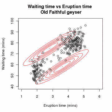
The steps of the EM algorithm on a two component Gaussian mixture model on the Old Faithful dataset

Let x=(x₁,x₂,…,x_n) be a sample of independent observations from a mixture of two multivariate normal distributions, and let z=(z₁,z₂,…,z_n) be the latent variables that determine the component from which the observation originates.^[3]

$X_i |(Z_i = 1) \sim \mathcal{N}_p(\boldsymbol{\mu}_1,\Sigma_1)$ and $X_i |(Z_i = 2) \sim \mathcal{N}_p(\boldsymbol{\mu}_2,\Sigma_2)$

where

$\operatorname{P} (Z_i = 1 ) = \tau_1 \,$ and $\operatorname{P} (Z_i=2) = \tau_2 = 1-\tau_1$

The aim is to estimate the unknown parameters representing the "mixing" value between the Gaussians and the means and standard deviations of each:

$\theta = \big( \boldsymbol{\tau},\boldsymbol{\mu}_1,\boldsymbol{\mu}_2,\Sigma_1,\Sigma_2 \big)$

where the likelihood function is:

$L(\theta;\mathbf{x},\mathbf{z}) = \prod_{i=1}^n \sum_{j=1}^2 \mathbb{I}(z_i=j) \ \tau_j \ f(\mathbf{x}_i;\boldsymbol{\mu}_j,\Sigma_j)$

where $\mathbb{I}$ is an indicator function and f is the probability density function of a multivariate normal. This may be rewritten in exponential family form:

$L(\theta;\mathbf{x},\mathbf{z}) = \exp \left\{ \sum_{i=1}^n \sum_{j=1}^2 \mathbb{I}(z_i=j) \big[ \log \tau_j -\tfrac{1}{2} \log |\Sigma_j| -\tfrac{1}{2}(\mathbf{x}_i-\boldsymbol{\mu}_j)^\top\Sigma_j^{-1} (\mathbf{x}_i-\boldsymbol{\mu}_j) -\tfrac{p}{2} \log(2\pi) \big] \right\}$

[edit] E-step

Given our current estimate of the parameters θ^(t), the conditional distribution of the Z_i is determined by Bayes theorem to be the proportional height of the normal density weighted by τ:

$T_{j,i}^{(t)} := \operatorname{P}(Z_i=j | X_i=\mathbf{x}_i ;\theta^{(t)}) = \frac{\tau_j^{(t)} \ f(\mathbf{x}_i;\boldsymbol{\mu}_j^{(t)},\Sigma_j^{(t)})}{\tau_1^{(t)} \ f(\mathbf{x}_i;\boldsymbol{\mu}_1^{(t)},\Sigma_1^{(t)}) + \tau_2^{(t)} \ f(\mathbf{x}_i;\boldsymbol{\mu}_2^{(t)},\Sigma_2^{(t)})}$ .

Thus, the E-step results in the function:

$Q(\theta|\theta^{(t)}) = \operatorname{E} [\log L(\theta;\mathbf{x},\mathbf{Z}) ] = \sum_{i=1}^n \sum_{j=1}^2 T_{j,i}^{(t)} \big[ \log \tau_j -\tfrac{1}{2} \log |\Sigma_j| -\tfrac{1}{2}(\mathbf{x}_i-\boldsymbol{\mu}_j)^\top\Sigma_j^{-1} (\mathbf{x}_i-\boldsymbol{\mu}_j) -\tfrac{p}{2} \log(2\pi) \big]$

[edit] M-step

The linear form of Q(θ|θ^(t)) means that determining the maximising values of θ is relatively straightforward. Firstly note that τ, (μ₁,Σ₁) and (μ₂,Σ₂) may be all maximised independently of each other since they all appear in separate linear terms.

Firstly, consider τ, which has the constraint τ₁ + τ₂=1:

$\boldsymbol{\tau}^{(t+1)} = \underset{\boldsymbol{\tau}} \operatorname{arg\,max}\ Q(\theta | \theta^{(t)} ) = \underset{\boldsymbol{\tau}} \operatorname{arg\,max} \ \left\{ \left[ \sum_{i=1}^n T_{1,i}^{(t)} \right] \log \tau_1 + \left[ \sum_{i=1}^n T_{2,i}^{(t)} \right] \log \tau_2 \right\}$

This has the same form as the MLE for the binomial distribution, so:

$\tau^{(t+1)}_j = \frac{\sum_{i=1}^n T_{j,i}^{(t)}}{\sum_{i=1}^n (T_{1,i}^{(t)} + T_{2,i}^{(t)} ) } = \frac{1}{n} \sum_{i=1}^n T_{j,i}^{(t)}$

For the next estimates of (μ₁,Σ₁):

$(\boldsymbol{\mu}_1^{(t+1)},\Sigma_1^{(t+1)}) = \underset{\boldsymbol{\mu}_1,\Sigma_1} \operatorname{arg\,max}\ Q(\theta | \theta^{(t)} ) = \underset{\boldsymbol{\mu}_1,\Sigma_1} \operatorname{arg\,max}\ \sum_{i=1}^n T_{1,i}^{(t)} \left\{ -\tfrac{1}{2} \log |\Sigma_1| -\tfrac{1}{2}(\mathbf{x}_i-\boldsymbol{\mu}_1)^\top\Sigma_1^{-1} (\mathbf{x}_i-\boldsymbol{\mu}_1) \right\}$

This has the same form as a weighted MLE for a normal distribution, so

$\boldsymbol{\mu}_1^{(t+1)} = \frac{\sum_{i=1}^n T_{1,i}^{(t)} \mathbf{x}_i}{\sum_{i=1}^n T_{1,i}^{(t)}}$ and $\Sigma_1^{(t+1)} = \frac{\sum_{i=1}^n T_{1,i}^{(t)} (\mathbf{x}_i - \boldsymbol{\mu}_1^{(t+1)})^\top (\mathbf{x}_i - \boldsymbol{\mu}_1^{(t+1)}) }{\sum_{i=1}^n T_{1,i}^{(t)}}$

and, by symmetry:

$\boldsymbol{\mu}_2^{(t+1)} = \frac{\sum_{i=1}^n T_{2,i}^{(t)} \mathbf{x}_i}{\sum_{i=1}^n T_{2,i}^{(t)}}$ and $\Sigma_2^{(t+1)} = \frac{\sum_{i=1}^n T_{2,i}^{(t)} (\mathbf{x}_i - \boldsymbol{\mu}_2^{(t+1)})^\top (\mathbf{x}_i - \boldsymbol{\mu}_2^{(t+1)}) }{\sum_{i=1}^n T_{2,i}^{(t)}}$ .

[edit] See also

[edit] Notes

^ Dempster, A.P.; Laird, N.M.; Rubin, D.B. (1977). "Maximum Likelihood from Incomplete Data via the EM Algorithm". Journal of the Royal Statistical Society. Series B (Methodological) 39 (1): 1–38. JSTOR: 2984875. MR 0501537.
^ ^a ^b Neal, Radford; Hinton, Geoffrey (1999). Michael I. Jordan. ed. "A view of the EM algorithm that justifies incremental, sparse, and other variants". Learning in Graphical Models (Cambridge, MA: MIT Press): 355–368. ISBN 0262600323. ftp://ftp.cs.toronto.edu/pub/radford/emk.pdf. Retrieved on 2009-03-22.
^ ^a ^b Hastie, Trevor; Tibshirani, Robert; Friedman, Jerome (2001). "8.5 The EM algorithm". The Elements of Statistical Learning. New York: Springer. pp. 236–243. ISBN 0-387-95284-5.
^ Jamshidian, Mortaza; Jennrich, Robert I. (1997). "Acceleration of the EM Algorithm by using Quasi-Newton Methods". Journal of the Royal Statistical Society: Series B (Statistical Methodology) 59 (2): 569–587. doi:10.1111/1467-9868.00083. MR 1452026.
^ Meng, Xiao-Li; Rubin, Donald B. (1993). "Maximum likelihood estimation via the ECM algorithm: A general framework". Biometrika 80 (2): 267–278. doi:10.1093/biomet/80.2.267. MR 1243503.

[edit] References

Robert Hogg, Joseph McKean and Allen Craig. Introduction to Mathematical Statistics. pp. 359-364. Upper Saddle River, NJ: Pearson Prentice Hall, 2005.
The on-line textbook: Information Theory, Inference, and Learning Algorithms, by David J.C. MacKay includes simple examples of the E-M algorithm such as clustering using the soft K-means algorithm, and emphasizes the variational view of the E-M algorithm.
A Gentle Tutorial of the EM Algorithm and its Application to Parameter Estimation for Gaussian Mixture and Hidden Markov Models, by Jeff Bilmes includes a simplified derivation of the EM equations for Gaussian Mixtures and Gaussian Mixture Hidden Markov Models.
Variational Algorithms for Approximate Bayesian Inference, by M. J. Beal includes comparisons of EM to Variational Bayesian EM and derivations of several models including Variational Bayesian HMMs.
The Expectation Maximization Algorithm, by Frank Dellaert, gives an easier explanation of EM algorithm in terms of lowerbound maximization.
The Expectation Maximization Algorithm: A short tutorial, A self contained derivation of the EM Algorithm by Sean Borman.

[edit] External links

Various 1D, 2D and 3D demonstrations of EM together with Mixture Modeling are provided as part of the paired SOCR activities and applets. These applets and activities show empirically the properties of the EM algorithm for parameter estimation in diverse settings.
Java code example
Another Java code example

[0] Dempster, A.P.; Laird, N.M.; Rubin, D.B. (1977). "Maximum Likelihood from Incomplete Data via the EM Algorithm". Journal of the Royal Statistical Society. Series B (Methodological) 39 (1): 1–38. JSTOR: 2984875. MR 0501537.

[neal1999-1] Neal, Radford; Hinton, Geoffrey (1999). Michael I. Jordan. ed. "A view of the EM algorithm that justifies incremental, sparse, and other variants". Learning in Graphical Models (Cambridge, MA: MIT Press): 355–368. ISBN 0262600323. ftp://ftp.cs.toronto.edu/pub/radford/emk.pdf. Retrieved on 2009-03-22.

[hastie2001-2] Hastie, Trevor; Tibshirani, Robert; Friedman, Jerome (2001). "8.5 The EM algorithm". The Elements of Statistical Learning. New York: Springer. pp. 236–243. ISBN 0-387-95284-5.

[3] Jamshidian, Mortaza; Jennrich, Robert I. (1997). "Acceleration of the EM Algorithm by using Quasi-Newton Methods". Journal of the Royal Statistical Society: Series B (Statistical Methodology) 59 (2): 569–587. doi:10.1111/1467-9868.00083. MR 1452026.

[4] Meng, Xiao-Li; Rubin, Donald B. (1993). "Maximum likelihood estimation via the ECM algorithm: A general framework". Biometrika 80 (2): 267–278. doi:10.1093/biomet/80.2.267. MR 1243503.

[1]

[2]

[3]

[4]

[5]

Expectation-maximization algorithm

From Wikipedia, the free encyclopedia

Contents

[edit] History

[edit] Description

[edit] Properties

[edit] Alternative description

[edit] Applications

[edit] Variants

[edit] Relation to variational Bayes methods

[edit] Example: Gaussian Mixture

[edit] E-step

[edit] M-step

[edit] See also

[edit] Notes

[edit] References

[edit] External links

Views

Personal tools

Navigation

Search

Interaction

Toolbox

Languages