Regression analysis

From Wikipedia, the free encyclopedia

In statistics, regression analysis refers to techniques for the modeling and analysis of numerical data consisting of values of a dependent variable (also called response variable or measurement) and of one or more independent variables (also known as explanatory variables or predictors). The dependent variable in the regression equation is modeled as a function of the independent variables, corresponding parameters ("constants"), and an error term. The error term is treated as a random variable. It represents unexplained variation in the dependent variable. The parameters are estimated so as to give a "best fit" of the data. Most commonly the best fit is evaluated by using the least squares method, but other criteria have also been used.

Regression can be used for prediction (including forecasting of time-series data), inference, hypothesis testing, and modeling of causal relationships. These uses of regression rely heavily on the underlying assumptions being satisfied. Regression analysis has been criticized as being misused for these purposes in many cases where the appropriate assumptions cannot be verified to hold.^[1]^[2] One factor contributing to the misuse of regression is that it can take considerably more skill to critique a model than to fit a model.^[3]

[edit] History of regression analysis

The earliest form of regression was the method of least squares, which was published by Legendre in 1805,^[4] and by Gauss in 1809.^[5] The term “least squares” is from Legendre’s term, moindres carrés. However, Gauss claimed that he had known the method since 1795.

Legendre and Gauss both applied the method to the problem of determining, from astronomical observations, the orbits of bodies about the Sun. Euler had worked on the same problem (1748) without success.^{[citation needed]} Gauss published a further development of the theory of least squares in 1821,^[6] including a version of the Gauss–Markov theorem.

The term "regression" was coined by Francis Galton, a cousin of Charles Darwin, in the nineteenth century to describe a biological phenomenon. The phenomenon was that the heights of descendants of tall ancestors tend to regress down towards a normal average.^[7] For Galton, regression had only this biological meaning, but his work^[8] was later extended by Udny Yule and Karl Pearson to a more general statistical context.^[9] At the present time, the term "regression" is often synonymous with "least-squares curve fitting".

[edit] Underlying assumptions

Classical assumptions for regression analysis include:

The sample must be representative of the population for the inference prediction.
The error is assumed to be a random variable with a mean of zero conditional on the explanatory variables.
The independent variables are error-free. If this is not so, modeling may be done using errors-in-variables model techniques.
The predictors must be linearly independent, i.e. it must not be possible to express any predictor as a linear combination of the others. See Multicollinearity.
The errors are uncorrelated, that is, the variance-covariance matrix of the errors is diagonal and each non-zero element is the variance of the error.
The variance of the error is constant across observations (homoscedasticity). If not, weighted least squares or other methods might be used.

These are sufficient (but not all necessary) conditions for the least-squares estimator to possess desirable properties, in particular, these assumptions imply that the parameter estimates will be unbiased, consistent, and efficient in the class of linear unbiased estimators. Many of these assumptions may be relaxed in more advanced treatments.

Assumptions include the geometrical support of the variables (Cressie, 1996). Independent and dependant variables often refer to values measured at point locations. There may be spatial trends and spatial autocorrelation in the variables that violates statistical assumptions of regression. Geographic weighted regression is one technique to deal with such data (Fotheringham et al., 2002). Also, variables may include values aggregated by areas. With aggregated data the Modifiable Areal Unit Problem can cause extreme variation in regression parameters (Fotheringham and Wong, 1991). When analyzing data aggregated by political boundaries, postal codes or census areas results may be very different with a different choice of units.

[edit] Regression equation

It is convenient to assume an environment in which an experiment is performed: the dependent variable is then outcome of a measurement.

The regression equation deals with the following variables:

The unknown parameters denoted as β. This may be a scalar or a vector of length k.
The independent variables, X.
The dependent variable, Y.

Regression equation is a function of variables X and β.

$Y = f (\mathbf {X}, \boldsymbol{\beta} )$

The user of regression analysis must make an intelligent guess about this function. Sometimes the form of this function is known, sometimes he must apply a trial and error process.

Assume now that the vector of unknown parameters, β is of length k. In order to perform a regression analysis the user must provide information about the dependent variable Y:

If the user performs the measurement N times, where N < k, regression analysis cannot be performed: there is not provided enough information to do so.
If the user performs N independent measurements, where N = k, then the problem reduces to solving a set of N equations with N unknowns β.
If, on the other hand, the user provides results of N independent measurements, where N > k, regression analysis can be performed. Such a system is also called an overdetermined system;

In the last case the regression analysis provides the tools for:

finding a solution for unknown parameters β that will, for example, minimize the distance between the measured and predicted values of the dependent variable Y (also known as method of least squares).
under certain statistical assumptions the regression analysis uses the surplus of information to provide statistical information about the unknown parameters β and predicted values of the dependent variable Y.

[edit] Independent measurements

Quantitatively, this is explained by the following example: Consider a regression model with, say, three unknown parameters β₀, β₁ and β₂. An experimenter performed 10 repeated measurements at exactly the same value of independent variables X. In this case regression analysis fails to give a unique value for the three unknown parameters: the experimenter did not provide enough information. The best one can do is to calculate the average value of the dependent variable Y and its standard deviation.

If the experimenter had performed five measurements at X₁, four at X₂ and one at X₃, where X₁, X₂ and X₃ are different values of the independent variable X then regression analysis would provide a unique solution to unknown parameters β.

In the case of general linear regression (see below) the above statement is equivalent to the requirement that matrix X^TX is regular (that is: it has an inverse matrix).

[edit] Statistical assumptions

When the number of measurements, N, is larger than the number of unknown parameters, k, and the measurement errors ε_i (see below) are normally distributed then the excess of information contained in (N - k) measurements is used to make the following statistical predictions about the unknown parameters:

confidence intervals of unknown parameters.

[edit] Linear regression

Main article: Linear regression

In linear regression, the model specification is that the dependent variable, $y i$ is a linear combination of the parameters (but need not be linear in the independent variables). For example, in simple linear regression for modeling $N$ data points there is one independent variable: $x i$ , and two parameters, $β 0$ and $β 1$ :

straight line: $y_i=\beta_0 +\beta_1 x_i +\varepsilon_i,\quad i=1,\dots,N\!$

In multiple linear regression, there are several independent variables or functions of independent variables. For example, adding a term in x_i² to the preceding regression gives:

parabola: $y_i=\beta_0 +\beta_1 x_i +\beta_2 x_i^2+\varepsilon_i,\ i=1,\dots,N\!$

This is still linear regression; although the expression on the right hand side is quadratic in the independent variable $x i$ , it is linear in the parameters $β 0$ , $β 1$ and $β 2 .$

In both cases, $\varepsilon_i$ is an error term and the subscript $i$ indexes a particular observation. Given a random sample from the population, we estimate the population parameters and obtain the sample linear regression model:

$y_i = \widehat{\beta}_0 + \widehat{\beta}_1 X_i + e_i$

The term $e i$ is the residual, $e_i = y_i - \widehat{y}_i$ . One method of estimation is ordinary least squares. This method obtains parameter estimates that minimize the sum of squared residuals, SSE:

$SSE=\sum_{i=1}^N e_i^2 \,$

Minimization of this function results in a set of normal equations, a set of simultaneous linear equations in the parameters, which are solved to yield the parameter estimators, $\widehat{\beta}_0, \widehat{\beta}_1$ . See regression coefficients for statistical properties of these estimators.

Illustration of linear regression on a data set.

In the case of simple regression, the formulas for the least squares estimates are

$\widehat{\beta_1}=\frac{\sum(x_i-\bar{x})(y_i-\bar{y})}{\sum(x_i-\bar{x})^2}\text{ and }\hat{\beta_0}=\bar{y}-\widehat{\beta_1}\bar{x}$

where $\bar{x}$ is the mean (average) of the $x$ values and $\bar{y}$ is the mean of the $y$ values. See linear least squares(straight line fitting) for a derivation of these formulas and a numerical example. Under the assumption that the population error term has a constant variance, the estimate of that variance is given by:

$\hat{\sigma}^2_\varepsilon = \frac{SSE}{N-2}.\,$

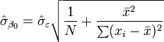
This is called the root mean square error (RMSE) of the regression. The standard errors of the parameter estimates are given by

$\hat\sigma_{\beta_0}=\hat\sigma_{\varepsilon} \sqrt{\frac{1}{N} + \frac{\bar{x}^2}{\sum(x_i-\bar x)^2}}$

$\hat\sigma_{\beta_1}=\hat\sigma_{\varepsilon} \sqrt{\frac{1}{\sum(x_i-\bar x)^2}}$

Under the further assumption that the population error term is normally distributed, the researcher can use these estimated standard errors to create confidence intervals and conduct hypothesis tests about the population parameters.

[edit] General linear data model

In the more general multiple regression model, there are p independent variables:

$y_i = \beta_0 + \beta_1 x_{1i} + \cdots + \beta_p x_{pi} + \varepsilon_i, \,$

The least square parameter estimates are obtained by p normal equations. The residual can be written as

$e_i=y_i - \hat\beta_0 - \hat\beta_1 x_1 - \cdots - \hat\beta_p x_p$

The normal equations are

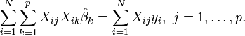
$\sum_{i=1}^N \sum_{k=1}^p X_{ij}X_{ik}\hat \beta_k=\sum_{i=1}^N X_{ij}y_i,\ j=1,\dots,p.\,$

In matrix notation, the normal equations are written as

$\mathbf{\left(X^TX\right)\hat \boldsymbol \beta=X^Ty}\,$

For a numerical example see linear regression (example).

[edit] Regression diagnostics

Once a regression model has been constructed, it may be important to confirm the goodness of fit of the model and the statistical significance of the estimated parameters. Commonly used checks of goodness of fit include the R-squared, analyses of the pattern of residuals and hypothesis testing. Statistical significance can be checked by an F-test of the overall fit, followed by t-tests of individual parameters.

Interpretations of these diagnostic tests rest heavily on the model assumptions. Although examination of the residuals can be used to invalidate a model, the results of a t-test or F-test are sometimes more difficult to interpret if the model's assumptions are violated. For example, if the error term does not have a normal distribution, in small samples the estimated parameters will not follow normal distributions, which complicates inference. With relatively large samples, however, a central limit theorem can be invoked such that hypothesis testing may proceed using asymptotic approximations.

[edit] Regression with limited dependent variables

The response variable may be non-continuous ("limited" to lie on some subset of the real line). For binary (zero or one) variables, if analysis proceeds with least-squares linear regression, the model is called the linear-probability model. Nonlinear models for binary dependent variables include the probit and logit model. The multivariate probit model makes it possible to estimate jointly the relationship between several binary dependent variables and some independent variables. For categorical variables with more than two values there is the multinomial logit. For ordinal variables with more than two values, there are the ordered logit and ordered probit models. Censored regression models may be used when the dependent variable is only sometimes observed, and Heckman correction type models may be used when the sample is not randomly selected from the population of interest. An alternative to such procedures is linear regression based on polychoric or polyserial correlations between the categorical variables. Such procedures differ in the assumptions made about the distribution of the variables in the population. If the variable is positive with low values and represents the repetition of the occurrence of an event, count models like the Poisson regression or the negative binomial model may be used

[edit] Interpolation and extrapolation

Regression models predict a value of the $y$ variable given known values of the $x$ variables. If the prediction is to be done within the range of values of the $x$ variables used to construct the model this is known as interpolation. Prediction outside the range of the data used to construct the model is known as extrapolation and it is more risky.

[edit] Nonlinear regression

Main article: Nonlinear regression

When the model function is not linear in the parameters the sum of squares must be minimized by an iterative procedure. This introduces many complications which are summarized in Differences between linear and non-linear least squares

[edit] Other methods

Although the parameters of a regression model are usually estimated using the method of least squares, other methods which have been used include:

Bayesian methods, e.g. Bayesian linear regression
Minimization of absolute deviations, leading to quantile regression
Nonparametric regression. This approach requires a large number of observations, as the data are used to build the model structure as well as estimate the model parameters. They are usually computationally intensive.

[edit] See also

Statistics portal

Confidence interval
Confidence region
Extrapolation
Kriging (a linear least squares estimation algorithm)
Forecasting
Prediction interval
Statistics
Trend estimation
Robust regression
Multivariate normal distribution
Important publications in regression analysis
Multivariate adaptive regression splines
Segmented regression

[edit] References

^ Richard A. Berk, Regression Analysis: A Constructive Critique, Sage Publications (2004)
^ David A. Freedman, Statistical Models: Theory and Practice, Cambridge University Press (2005)
^ [1] R. Dennis Cook; Sanford Weisberg "Criticism and Influence Analysis in Regression", Sociological Methodology, Vol. 13. (1982), pp. 313-361.
^ A.M. Legendre. Nouvelles méthodes pour la détermination des orbites des comètes (1805). “Sur la Méthode des moindres quarrés” appears as an appendix.
^ C.F. Gauss. Theoria Motus Corporum Coelestium in Sectionibus Conicis Solem Ambientum. (1809)
^ C.F. Gauss. Theoria combinationis observationum erroribus minimis obnoxiae. (1821/1823)
^ Mogull, Robert G. (2004). Second-Semester Applied Statistics. Kendall/Hunt Publishing Company. pp. 59. ISBN 0-7575-1181-3.
^ Francis Galton. "Typical laws of heredity", Nature 15 (1877), 492-495, 512-514, 532-533. (Galton uses the term "reversion" in this paper, which discusses the size of peas.); Francis Galton. Presidential address, Section H, Anthropology. (1885) (Galton uses the term "regression" in this paper, which discusses the height of humans.)
^ G. Udny Yule. "On the Theory of Correlation", J. Royal Statist. Soc., 1897, p. 812-54. Karl Pearson, G. U. Yule, Norman Blanchard, and Alice Lee. "The Law of Ancestral Heredity", Biometrika (1903). In the work of Yule and Pearson, the joint distribution of the response and explanatory variables is assumed to be Gaussian. This assumption was weakened by R.A. Fisher in his works of 1922 and 1925 (R.A. Fisher, "The goodness of fit of regression formulae, and the distribution of regression coefficients", J. Royal Statist. Soc., 85, 597-612 from 1922 and Statistical Methods for Research Workers from 1925). Fisher assumed that the conditional distribution of the response variable is Gaussian, but the joint distribution need not be. In this respect, Fisher's assumption is closer to Gauss's formulation of 1821.

Audi, R., Ed. (1996). "curve fitting problem," The Cambridge Dictionary of Philosophy. Cambridge, Cambridge University Press. pp.172-173.
William H. Kruskal and Judith M. Tanur, ed. (1978), "Linear Hypotheses," International Encyclopedia of Statistics. Free Press, v. 1,

Evan J. Williams, "I. Regression," pp. 523-41.

Julian C. Stanley, "II. Analysis of Variance," pp. 541-554.

Lindley, D.V. (1987). "Regression and correlation analysis," New Palgrave: A Dictionary of Economics, v. 4, pp. 120-23.
Birkes, David and Yadolah Dodge, Alternative Methods of Regression. ISBN 0-471-56881-3
Chatfield, C. (1993) "Calculating Interval Forecasts," Journal of Business and Economic Statistics, 11. pp. 121-135.
Draper, N.R. and Smith, H. (1998).Applied Regression Analysis Wiley Series in Probability and Statistics
Fox, J. (1997). Applied Regression Analysis, Linear Models and Related Methods. Sage
Hardle, W., Applied Nonparametric Regression (1990), ISBN 0-521-42950-1
Meade, N. and T. Islam (1995) "Prediction Intervals for Growth Curve Forecasts," Journal of Forecasting, 14, pp. 413-430.
Munro, Barbara Hazard (2005) "Statistical Methods for Health Care Research" Lippincott Williams & Wilkins, 5th ed.
Gujarati, Basic Econometrics, 4th edition
Sykes, A.O. "An Introduction to Regression Analysis" (Inaugural Coase Lecture)
S. Kotsiantis, D. Kanellopoulos, P. Pintelas, Local Additive Regression of Decision Stumps, Lecture Notes in Artificial Intelligence, Springer-Verlag, Vol. 3955, SETN 2006, pp. 148 – 157, 2006
S. Kotsiantis, P. Pintelas, Selective Averaging of Regression Models, Annals of Mathematics, Computing & TeleInformatics, Vol 1, No 3, 2005, pp. 66-75
N. Cressie (1996) Change of Support and the Modiable Areal Unit Problem. Geographical Systems 3:159-180.
A.S. Fotheringham, C. Brunsdon, and M. Charlton. (2002) Geographically weighted regression: the analysis of spatially varying relationships. Wiley.
A.S. Fotheringham and D. Wong. (1991) The modifiable areal unit problem in multivariate statistical analysis. Environment and Planning A, 23(1):1025-1044.

[edit] Software

All major statistical-software packages perform the common types of regression analysis correctly and in a user-friendly way. Simple linear regression can be done in some spreadsheet applications. There are a number of software programs that perform specialized forms of regression, and experts may choose to write their own code to using statistical programming languages or numerical analysis software.

[edit] External links

Wikimedia Commons has media related to: Regression analysis

Regression Analysis
Regression Analysis Tool Online Article on linear regression with a Regression Analysis Tool
Curvefit: A complete guide to nonlinear regression - Online textbook
Exegeses on Linear Models - Some comments on linear regression models by Bill Venables.
Perpendicular Regression of a Line at MathPages
Regression of Weakly Correlated Data - How linear regression mistakes can appear when Y-range is much smaller than X-range
Matlab SUrrogate MOdeling Toolbox - SUMO Toolbox - Matlab code for Active Learning + Model Selection + Surrogate Model Regression
Zunzun.com Online curve and surface fitting application

[Berk-0] Richard A. Berk, Regression Analysis: A Constructive Critique, Sage Publications (2004)

[1] David A. Freedman, Statistical Models: Theory and Practice, Cambridge University Press (2005)

[2] [1] R. Dennis Cook; Sanford Weisberg "Criticism and Influence Analysis in Regression", Sociological Methodology, Vol. 13. (1982), pp. 313-361.

[Legendre-3] A.M. Legendre. Nouvelles méthodes pour la détermination des orbites des comètes (1805). “Sur la Méthode des moindres quarrés” appears as an appendix.

[Gauss-4] C.F. Gauss. Theoria Motus Corporum Coelestium in Sectionibus Conicis Solem Ambientum. (1809)

[Gauss2-5] C.F. Gauss. Theoria combinationis observationum erroribus minimis obnoxiae. (1821/1823)

[6] Mogull, Robert G. (2004). Second-Semester Applied Statistics. Kendall/Hunt Publishing Company. pp. 59. ISBN 0-7575-1181-3.

[7] Francis Galton. "Typical laws of heredity", Nature 15 (1877), 492-495, 512-514, 532-533. (Galton uses the term "reversion" in this paper, which discusses the size of peas.); Francis Galton. Presidential address, Section H, Anthropology. (1885) (Galton uses the term "regression" in this paper, which discusses the height of humans.)

[8] G. Udny Yule. "On the Theory of Correlation", J. Royal Statist. Soc., 1897, p. 812-54. Karl Pearson, G. U. Yule, Norman Blanchard, and Alice Lee. "The Law of Ancestral Heredity", Biometrika (1903). In the work of Yule and Pearson, the joint distribution of the response and explanatory variables is assumed to be Gaussian. This assumption was weakened by R.A. Fisher in his works of 1922 and 1925 (R.A. Fisher, "The goodness of fit of regression formulae, and the distribution of regression coefficients", J. Royal Statist. Soc., 85, 597-612 from 1922 and Statistical Methods for Research Workers from 1925). Fisher assumed that the conditional distribution of the response variable is Gaussian, but the joint distribution need not be. In this respect, Fisher's assumption is closer to Gauss's formulation of 1821.

[1]

[2]

[3]

[4]

[5]

[6]

[7]

[8]

[9]

Regression analysis

From Wikipedia, the free encyclopedia

Contents

[edit] History of regression analysis

[edit] Underlying assumptions

[edit] Regression equation

[edit] Independent measurements

[edit] Statistical assumptions

[edit] Linear regression

[edit] General linear data model

[edit] Regression diagnostics

[edit] Regression with limited dependent variables

[edit] Interpolation and extrapolation

[edit] Nonlinear regression

[edit] Other methods

[edit] See also

[edit] References

[edit] Software

[edit] External links

Views

Personal tools

Navigation

Search

Interaction

Toolbox

Languages