Wavelet

From Wikipedia, the free encyclopedia

This page may be too technical for a general audience. Please help improve the page by providing more context and better explanations of technical details, even for subjects that are inherently technical.

A non-technical definition of a wavelet is that it is a wave with an amplitude that starts out at zero, increases, and then decreases back to zero. It can typically be visualized as a "brief oscillation" like one might see recorded by a seismograph or heart monitor. Generally, wavelets are purposefully crafted to have specific properties that make them useful for signal processing. Wavelets can be combined, using a "shift, multiply and sum" technique called convolution, with portions of an unknown signal to extract information from the unknown signal. For example, a wavelet could be created to have a frequency of "Middle C" and a short duration of roughly a 32nd note. If this wavelet were to be convolved at periodic intervals with a signal created from the recording of a song, then the results of these convolutions would be useful for determining when the "Middle C" note was being played in the song. Mathematically the wavelet will resonate if the unknown signal contains information of similar frequency - just as a tuning fork physically resonates with sound waves of its specific tuning frequency. This concept of resonance is at the core of many practical applications of wavelet theory.

As wavelets are a mathematical tool they can be used to extract information from many different kinds of data, including - but certainly not limited to - audio signals and images. Sets of wavelets are generally needed to fully analyze data. A set of "complementary" wavelets will deconstruct data without gaps or overlap so that the deconstruction process is mathematically reversible. Thus, sets of complementary wavelets are useful in wavelet based compression/decompression algorithms where it is desirable to recover the original information with minimal loss.

A broader and more rigorous definition of a wavelet is that it is a mathematical function used to divide a given function or continuous-time signal into different scale components. Usually one can assign a frequency range to each scale component. Each scale component can then be studied with a resolution that matches its scale. A wavelet transform is the representation of a function by wavelets. The wavelets are scaled and translated copies (known as "daughter wavelets") of a finite-length or fast-decaying oscillating waveform (known as the "mother wavelet"). Wavelet transforms have advantages over traditional Fourier transforms for representing functions that have discontinuities and sharp peaks, and for accurately deconstructing and reconstructing finite, non-periodic and/or non-stationary signals.

In formal terms, this representation is a wavelet series representation of a square-integrable function with respect to either a complete, orthonormal set of basis functions, or an overcomplete set of Frame of a vector space (also known as a Riesz basis), for the Hilbert space of square integrable functions.

Wavelet transforms are classified into discrete wavelet transforms (DWTs) and continuous wavelet transforms (CWTs). Note that both DWT and CWT are continuous-time (analog) transforms. They can be used to represent continuous-time (analog) signals. CWTs operate over every possible scale and translation whereas DWTs use a specific subset of scale and translation values or representation grid.

The word wavelet is due to Morlet and Grossmann in the early 1980s. They used the French word ondelette, meaning "small wave". Soon it was transferred to English by translating "onde" into "wave", giving "wavelet".

[edit] Wavelet theory

Wavelet theory is applicable to several subjects. All wavelet transforms may be considered forms of time-frequency representation for continuous-time (analog) signals and so are related to harmonic analysis. Almost all practically useful discrete wavelet transforms use discrete-time filterbanks. These filter banks are called the wavelet and scaling coefficients in wavelets nomenclature. These filterbanks may contain either finite impulse response (FIR) or infinite impulse response (IIR) filters. The wavelets forming a CWT are subject to the uncertainty principle of Fourier analysis respective sampling theory: Given a signal with some event in it, one cannot assign simultaneously an exact time and frequency response scale to that event. The product of the uncertainties of time and frequency response scale has a lower bound. Thus, in the scaleogram of a continuous wavelet transform of this signal, such an event marks an entire region in the time-scale plane, instead of just one point. Also, discrete wavelet bases may be considered in the context of other forms of the uncertainty principle.

Wavelet transforms are broadly divided into three classes: continuous, discrete and multiresolution-based.

[edit] Continuous wavelet transforms (Continuous Shift & Scale Parameters)

In continuous wavelet transforms, a given signal of finite energy is projected on a continuous family of frequency bands (or similar subspaces of the L^p function space $L^2(\R)$ ). For instance the signal may be represented on every frequency band of the form $[f,2 f]$ for all positive frequencies f>0. Then, the original signal can be reconstructed by a suitable integration over all the resulting frequency components.

The frequency bands or subspaces (sub-bands) are scaled versions of a subspace at scale 1. This subspace in turn is in most situations generated by the shifts of one generating function $\psi \in L^2(\R)$ , the mother wavelet. For the example of the scale one frequency band $[1,2]$ this function is

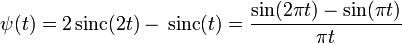
$\psi(t)=2\,\operatorname{sinc}(2t)-\,\operatorname{sinc}(t)=\frac{\sin(2\pi t)-\sin(\pi t)}{\pi t}$

with the (normalized) sinc function. Other example mother wavelets are:

Meyer

Morlet

Mexican Hat

The subspace of scale a or frequency band $[1/a,\,2/a]$ is generated by the functions (sometimes called child wavelets)

$\psi_{a,b} (t) = \frac1{\sqrt a }\psi \left( \frac{t - b}{a} \right)$ ,

where a is positive and defines the scale and b is any real number and defines the shift. The pair (a,b) defines a point in the right halfplane $\R_+\times \R$ .

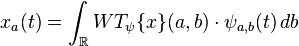
The projection of a function x onto the subspace of scale a then has the form

$x_a(t)=\int_\R WT_\psi\{x\}(a,b)\cdot\psi_{a,b}(t)\,db$

with wavelet coefficients

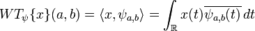$WT_\psi\{x\}(a,b)=\langle x,\psi_{a,b}\rangle=\int_\R x(t)\overline{\psi_{a,b}(t)}\,dt$ .

See a list of some Continuous wavelets.

For the analysis of the signal x, one can assemble the wavelet coefficients into a scaleogram of the signal.

[edit] Discrete wavelet transforms (Discrete Shift & Scale parameters)

It is computationally impossible to analyze a signal using all wavelet coefficients, so one may wonder if it is sufficient to pick a discrete subset of the upper halfplane to be able to reconstruct a signal from the corresponding wavelet coefficients. One such system is the affine system for some real parameters a>1, b>0. The corresponding discrete subset of the halfplane consists of all the points $(a^m, n\,a^m b)$ with integers $m,n\in\Z^2$ . The corresponding baby wavelets are now given as

ψ m, n (t) = a - m / 2 ψ(a - m t - n b)

.

A sufficient condition for the reconstruction of any signal x of finite energy by the formula

$x(t)=\sum_{m\in\Z}\sum_{n\in\Z}\langle x,\,\psi_{m,n}\rangle\cdot\psi_{m,n}(t)$

is that the functions $\{\psi_{m,n}:m,n\in\Z^2\}$ form a tight frame of $L^2(\R)$ .

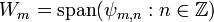
[edit] Multiresolution discrete wavelet transforms

D4 wavelet

In any discretised wavelet transform, there are only a finite number of wavelet coefficients for each bounded rectangular region in the upper halfplane. Still, each coefficient requires the evaluation of an integral. To avoid this numerical complexity, one needs one auxiliary function, the father wavelet $\phi\in L^2(\R)$ . Further, one has to restrict a to be an integer. A typical choice is a=2 and b=1. The most famous pair of father and mother wavelets is the Daubechies 4 tap wavelet.

From the mother and father wavelets one constructs the subspaces

$V_m=\operatorname{span}(\phi_{m,n}:n\in\Z)$ , where

φ m, n (t) = 2 - m / 2 φ(2 - m t - n)

and

$W_m=\operatorname{span}(\psi_{m,n}:n\in\Z)$ , where

ψ m, n (t) = 2 - m / 2 ψ(2 - m t - n)

.

From these one requires that the sequence

$\{0\}\subset\dots\subset V_1\subset V_0\subset V_{-1}\subset\dots\subset L^2(\R)$

forms a multiresolution analysis of $L^2(\R)$ and that the subspaces $\dots,W_1,W_0,W_{-1},\dots\dots$ are the orthogonal "differences" of the above sequence, that is, $W m$ is the orthogonal complement of $V m$ inside the subspace $V m - 1$ . In analogy to the sampling theorem one may conclude that the space $V m$ with sampling distance $2 m$ more or less covers the frequency baseband from 0 to $2 - m - 1$ . As orthogonal complement, $W m$ roughly covers the band $[2 - m - 1,2 - m]$ .

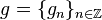From those inclusions and orthogonality relations follows the existence of sequences $h=\{h_n\}_{n\in\Z}$ and $g=\{g_n\}_{n\in\Z}$ that satisfy the identities

$h_n=\langle\phi_{0,0},\,\phi_{-1,n}\rangle$ and $\phi(t)=\sqrt2 \sum_{n\in\Z} h_n\phi(2t-n)$

and

$g_n=\langle\psi_{0,0},\,\phi_{-1,n}\rangle$ and $\psi(t)=\sqrt2 \sum_{n\in\Z} g_n\phi(2t-n)$ .

The second identity of the first pair is a refinement equation for the father wavelet $φ$ . Both pairs of identities form the basis for the algorithm of the fast wavelet transform.

[edit] Mother wavelet

For practical applications, and for efficiency reasons, one prefers continuously differentiable functions with compact support as mother (prototype) wavelet (functions). However, to satisfy analytical requirements (in the continuous WT) and in general for theoretical reasons, one chooses the wavelet functions from a subspace of the space 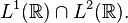$L^1(\R)\cap L^2(\R).$ This is the space of measurable functions that are absolutely and square integrable:

$\int_{-\infty}^{\infty} |\psi (t)|\, dt <\infty$ and $\int_{-\infty}^{\infty} |\psi (t)|^2 \, dt <\infty.$

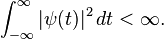
Being in this space ensures that one can formulate the conditions of zero mean and square norm one:

$\int_{-\infty}^{\infty} \psi (t)\, dt = 0$ is the condition for zero mean, and

$\int_{-\infty}^{\infty} |\psi (t)|^2\, dt = 1$ is the condition for square norm one.

For $ψ$ to be a wavelet for the continuous wavelet transform (see there for exact statement), the mother wavelet must satisfy an admissibility criterion (loosely speaking, a kind of half-differentiability) in order to get a stably invertible transform.

For the discrete wavelet transform, one needs at least the condition that the wavelet series is a representation of the identity in the space $L^2(\R)$ . Most constructions of discrete WT make use of the multiresolution analysis, which defines the wavelet by a scaling function. This scaling function itself is solution to a functional equation.

In most situations it is useful to restrict $ψ$ to be a continuous function with a higher number M of vanishing moments, i.e. for all integer m<M

$\int_{-\infty}^{\infty} t^m\,\psi (t)\, dt = 0.$

Some example mother wavelets are:

Meyer

Morlet

Mexican Hat

The mother wavelet is scaled (or dilated) by a factor of $a$ and translated (or shifted) by a factor of $b$ to give (under Morlet's original formulation):

$\psi _{a,b} (t) = {1 \over {\sqrt a }}\psi \left( {{{t - b} \over a}} \right).$

For the continuous WT, the pair (a,b) varies over the full half-plane $\R_+\times\R$ ; for the discrete WT this pair varies over a discrete subset of it, which is also called affine group.

These functions are often incorrectly referred to as the basis functions of the (continuous) transform. In fact, as in the continuous Fourier transform, there is no basis in the continuous wavelet transform. Time-frequency interpretation uses a subtly different formulation (after Delprat).

[edit] Comparisons with Fourier Transform (Continuous-Time)

The wavelet transform is often compared with the Fourier transform, in which signals are represented as a sum of sinusoids. The main difference is that wavelets are localized in both time and frequency whereas the standard Fourier transform is only localized in frequency. The Short-time Fourier transform (STFT) is also time and frequency localized but there are issues with the frequency time resolution and wavelets often give a better signal representation using Multiresolution analysis.

The discrete wavelet transform is also less computationally complex, taking O(N) time as compared to O(N log N) for the fast Fourier transform. This computational advantage is not inherent to the transform, but reflects the choice of a logarithmic division of frequency, in contrast to the equally spaced frequency divisions of the FFT.

[edit] Definition of a wavelet

There are a number of ways of defining a wavelet (or a wavelet family).

[edit] Scaling filter

The wavelet is entirely defined by the scaling filter - a low-pass finite impulse response (FIR) filter of length 2N and sum 1. In biorthogonal wavelets, separate decomposition and reconstruction filters are defined.

For analysis the high pass filter is calculated as the quadrature mirror filter of the low pass, and reconstruction filters the time reverse of the decomposition.

Daubechies and Symlet wavelets can be defined by the scaling filter.

[edit] Scaling function

Wavelets are defined by the wavelet function $ψ(t)$ (i.e. the mother wavelet) and scaling function $φ(t)$ (also called father wavelet) in the time domain.

The wavelet function is in effect a band-pass filter and scaling it for each level halves its bandwidth. This creates the problem that in order to cover the entire spectrum, an infinite number of levels would be required. The scaling function filters the lowest level of the transform and ensures all the spectrum is covered. See [1] for a detailed explanation.

For a wavelet with compact support, $φ(t)$ can be considered finite in length and is equivalent to the scaling filter g.

Meyer wavelets can be defined by scaling functions

[edit] Wavelet function

The wavelet only has a time domain representation as the wavelet function $ψ(t)$ .

For instance, Mexican hat wavelets can be defined by a wavelet function. See a list of a few Continuous wavelets.

[edit] Applications of Discrete Wavelet Transform

Generally, an approximation to DWT is used for data compression if signal is already sampled, and the CWT for signal analysis. Thus, DWT approximation is commonly used in engineering and computer science, and the CWT in scientific research.

Wavelet transforms are now being adopted for a vast number of applications, often replacing the conventional Fourier Transform. Many areas of physics have seen this paradigm shift, including molecular dynamics, ab initio calculations, astrophysics, density-matrix localisation, seismic geophysics, optics, turbulence and quantum mechanics. This change has also occurred in image processing, blood-pressure, heart-rate and ECG analyses, DNA analysis, protein analysis, climatology, general signal processing, speech recognition, computer graphics and multifractal analysis. In computer vision and image processing, the notion of scale-space representation and Gaussian derivative operators is regarded as a canonical multi-scale representation.

One use of wavelet approximation is in data compression. Like some other transforms, wavelet transforms can be used to transform data, then encode the transformed data, resulting in effective compression. For example, JPEG 2000 is an image compression standard that uses biorthogonal wavelets. This means that although the frame is overcomplete, it is a tight frame (see types of Frame of a vector space), and the same frame functions (except for conjugation in the case of complex wavelets) are used for both analysis and synthesis, i.e., in both the forward and inverse transform. For details see wavelet compression.

A related use is that of smoothing/denoising data based on wavelet coefficient thresholding, also called wavelet shrinkage. By adaptively thresholding the wavelet coefficients that correspond to undesired frequency components smoothing and/or denoising operations can be performed.

Wavelet transforms are also starting to be used for communication applications. Wavelet OFDM is the basic modulation scheme used in HD-PLC (a powerline communications technology developed by Panasonic), and in one of the optional modes included in the IEEE P1901 draft standard. The advantage of Wavelet OFDM over traditional FFT OFDM systems is that Wavelet can achieve deeper notches and that it does not require a Guard Interval (which usually represents significant overhead in FFT OFDM systems)^[1].

[edit] History

The development of wavelets can be linked to several separate trains of thought, starting with Haar's work in the early 20th century. Notable contributions to wavelet theory can be attributed to Zweig’s discovery of the continuous wavelet transform in 1975 (originally called the cochlear transform and discovered while studying the reaction of the ear to sound)^[2], Pierre Goupillaud, Grossmann and Morlet's formulation of what is now known as the CWT (1982), Jan-Olov Strömberg's early work on discrete wavelets (1983), Daubechies' orthogonal wavelets with compact support (1988), Mallat's multiresolution framework (1989), Nathalie Delprat's time-frequency interpretation of the CWT (1991), Newland's Harmonic wavelet transform (1993) and many others since.

[edit] Timeline

First wavelet (Haar wavelet) by Alfred Haar (1909)
Since the 1950s: George Zweig, Jean Morlet, Alex Grossmann
Since the 1980s: Yves Meyer, Stéphane Mallat, Ingrid Daubechies, Ronald Coifman, Victor Wickerhauser,

[edit] Wavelet Transforms

There are a large number of wavelet transforms each suitable for different applications. For a full list see list of wavelet-related transforms but the common ones are listed below:

[edit] Generalized Transforms

There are a number of generalized transforms of which the wavelet transform is a special case. For example, Joseph Segman introduced scale into the Heisenberg group, giving rise to a continuous transform space that is a function of time, scale, and frequency. The CWT is a two-dimensional slice through the resulting 3d time-scale-frequency volume.

Another example of a generalized transform is the chirplet transform in which the CWT is also a two dimensional slice through the chirplet transform.

An important application area for generalized transforms involves systems in which high frequency resolution is crucial. For example, darkfield electron optical transforms intermediate between direct and reciprocal space have been widely used in the harmonic analysis of atom clustering, i.e. in the study of crystals and crystal defects^[3]. Now that transmission electron microscopes are capable of providing digital images with picometer-scale information on atomic periodicity in nanostructure of all sorts, the range of pattern recognition^[4] and strain^[5]/metrology^[6] applications for intermediate transforms with high frequency resolution (like brushlets^[7] and ridgelets^[8]) is growing rapidly.

[edit] List of wavelets

[edit] Discrete wavelets

Beylkin (18)
BNC wavelets
Coiflet (6, 12, 18, 24, 30)
Cohen-Daubechies-Feauveau wavelet (Sometimes referred to as CDF N/P or Daubechies biorthogonal wavelets)
Daubechies wavelet (2, 4, 6, 8, 10, 12, 14, 16, 18, 20)
Binomial-QMF
Haar wavelet
Mathieu wavelet
Legendre wavelet
Villasenor wavelet
Symlet

[edit] Continuous wavelets

[edit] Real valued

[edit] Complex valued

[edit] See also

Chirplet transform
Curvelet
Filter banks
Fractional Fourier transform
Multiresolution analysis
Scale space
Short-time Fourier transform
Ultra wideband radio- transmits wavelets.

[edit] Notes

^ Recent Developments in the Standardization of Power Line Communications within the IEEE, (Galli, S. and Logvinov, O - IEEE Communications Magazine, July 2008)
^ http://scienceworld.wolfram.com/biography/Zweig.html Zweig, George Biography on Scienceworld.wolfram.com
^ P. Hirsch, A. Howie, R. Nicholson, D. W. Pashley and M. J. Whelan (1965/1977) Electron microscopy of thin crystals (Butterworths, London/Krieger, Malabar FLA) ISBN 0-88275-376-2
^ P. Fraundorf, J. Wang, E. Mandell and M. Rose (2006) Digital darkfield tableaus, Microscopy and Microanalysis 12:S2, 1010-1011 (cf. arXiv:cond-mat/0403017)
^ M. J. Hÿtch, E. Snoeck and R. Kilaas (1998) Quantitative measurement of displacement and strain fields from HRTEM micrographs, Ultramicroscopy 74:131-146.
^ Martin Rose (2006) Spacing measurements of lattice fringes in HRTEM image using digital darkfield decomposition (M.S. Thesis in Physics, U. Missouri - St. Louis)
^ F. G. Meyer and R. R. Coifman (1997) Applied and Computational Harmonic Analysis 4:147.
^ A. G. Flesia, H. Hel-Or, A. Averbuch, E. J. Candes, R. R. Coifman and D. L. Donoho (2001) Digital implementation of ridgelet packets (Academic Press, New York).

[edit] References

Paul S. Addison, The Illustrated Wavelet Transform Handbook, Institute of Physics, 2002, ISBN 0-7503-0692-0
Ingrid Daubechies, Ten Lectures on Wavelets, Society for Industrial and Applied Mathematics, 1992, ISBN 0-89871-274-2
A. N. Akansu and R. A. Haddad, Multiresolution Signal Decomposition: Transforms, Subbands, Wavelets, Academic Press, 1992, ISBN 0-12-047140-X
P. P. Vaidyanathan, Multirate Systems and Filter Banks, Prentice Hall, 1993, ISBN 0-13-605718-7
Mladen Victor Wickerhauser, Adapted Wavelet Analysis From Theory to Software, A K Peters Ltd, 1994, ISBN 1-56881-041-5
Gerald Kaiser, A Friendly Guide to Wavelets, Birkhauser, 1994, ISBN 0-8176-3711-7
Haar A., Zur Theorie der orthogonalen Funktionensysteme, Mathematische Annalen, 69, pp 331-371, 1910.
Ramazan Gençay, Faruk Selçuk and Brandon Whitcher, An Introduction to Wavelets and Other Filtering Methods in Finance and Economics, Academic Press, 2001, ISBN 0-12-279670-5
Donald B. Percival and Andrew T. Walden, Wavelet Methods for Time Series Analysis, Cambridge University Press, 2000, ISBN 0-5216-8508-7
Tony F. Chan and Jackie (Jianhong) Shen, Image Processing and Analysis - Variational, PDE, Wavelet, and Stochastic Methods, Society of Applied Mathematics, ISBN 089871589X (2005)
Stéphane Mallat, "A wavelet tour of signal processing" 2nd Edition, Academic Press, 1999, ISBN 0-12-466606-x
Barbara Burke Hubbard, "The World According to Wavelets: The Story of a Mathematical Technique in the Making", AK Peters Ltd, 1998, ISBN 1568810725, ISBN-13 978-1568810720

[edit] External links

Wikimedia Commons has media related to: Wavelet

Wavelet Digest
NASA Signal Processor featuring Wavelet methods Description of NASA Signal & Image Processing Software and Link to Download
1st NJIT Symposium on Wavelets (April 30, 1990) (First Wavelets Conference in USA)
Binomial-QMF Daubechies Wavelets
Wavelets made Simple
Course on Wavelets given at UC Santa Barbara, 2004
The Wavelet Tutorial by Polikar (Easy to understand when you have some background with fourier transforms!)
OpenSource Wavelet C++ Code
An Introduction to Wavelets
Wavelets for Kids (PDF file) (Introductory (for very smart kids!))
Link collection about wavelets
Gerald Kaiser's acoustic and electromagnetic wavelets
A really friendly guide to wavelets
Wavelet-based image annotation and retrieval
Very basic explanation of Wavelets and how FFT relates to it
A Practical Guide to Wavelet Analysis is very helpful, and the wavelet software in FORTRAN, IDL and MATLAB are freely available online. Note that the biased wavelet power spectrum needs to be rectified.
Where Is The Starlet? A dictionary of wavelet names.

[galli-0] Recent Developments in the Standardization of Power Line Communications within the IEEE, (Galli, S. and Logvinov, O - IEEE Communications Magazine, July 2008)

[1] ttp://scienceworld.wolfram.com/biography/Zweig.html Zweig, George Biography on Scienceworld.wolfram.com

[2] P. Hirsch, A. Howie, R. Nicholson, D. W. Pashley and M. J. Whelan (1965/1977) Electron microscopy of thin crystals (Butterworths, London/Krieger, Malabar FLA) ISBN 0-88275-376-2

[3] P. Fraundorf, J. Wang, E. Mandell and M. Rose (2006) Digital darkfield tableaus, Microscopy and Microanalysis 12:S2, 1010-1011 (cf. arXiv:cond-mat/0403017)

[4] M. J. Hÿtch, E. Snoeck and R. Kilaas (1998) Quantitative measurement of displacement and strain fields from HRTEM micrographs, Ultramicroscopy 74:131-146.

[5] Martin Rose (2006) Spacing measurements of lattice fringes in HRTEM image using digital darkfield decomposition (M.S. Thesis in Physics, U. Missouri - St. Louis)

[6] F. G. Meyer and R. R. Coifman (1997) Applied and Computational Harmonic Analysis 4:147.

[7] A. G. Flesia, H. Hel-Or, A. Averbuch, E. J. Candes, R. R. Coifman and D. L. Donoho (2001) Digital implementation of ridgelet packets (Academic Press, New York).

[1]

[2]

[3]

[4]

[5]

[6]

[7]

[8]