Particle swarm optimization

From Wikipedia, the free encyclopedia

Particle swarm optimization (PSO) is a swarm intelligence based algorithm to find a solution to an optimization problem in a search space, or model and predict social behavior in the presence of objectives.

[edit] Overview

Particle swarm optimization is a stochastic, population-based computer algorithm for problem solving. It is a kind of swarm intelligence that is based on social-psychological principles and provides insights into social behavior, as well as contributing to engineering applications. The particle swarm optimization algorithm was first described in 1995 by James Kennedy and Russell C. Eberhart. The techniques have evolved greatly since then, and the original version of the algorithm is barely recognizable in the current ones.

Social influence and social learning enable a person to maintain cognitive consistency. People solve problems by talking with other people about them, and as they interact their beliefs, attitudes, and behaviors change; the changes could typically be depicted as the individuals moving toward one another in a socio-cognitive space.

The particle swarm simulates this kind of social optimization. A problem is given, and some way to evaluate a proposed solution to it exists in the form of a fitness function. A communication structure or social network is also defined, assigning neighbors for each individual to interact with. Then a population of individuals defined as random guesses at the problem solutions is initialized. These individuals are candidate solutions. They are also known as the particles, hence the name particle swarm. An iterative process to improve these candidate solutions is set in motion. The particles iteratively evaluate the fitness of the candidate solutions and remember the location where they had their best success. The individual's best solution is called the particle best or the local best. Each particle makes this information available to their neighbors. They are also able to see where their neighbors have had success. Movements through the search space are guided by these successes, with the population usually converging, by the end of a trial, on a problem solution better than that of non-swarm approach using the same methods.

The swarm is typically modelled by particles in multidimensional space that have a position and a velocity. These particles fly through hyperspace (i.e., $\mathbb{R}^n$ ) and have two essential reasoning capabilities: their memory of their own best position and knowledge of the global or their neighborhood's best. In a minimization optimization problem, problems are formulated so that "best" simply means the position with the smallest objective value. Members of a swarm communicate good positions to each other and adjust their own position and velocity based on these good positions. So a particle has the following information to make a suitable change in its position and velocity:

A global best that is known to all and immediately updated when a new best position is found by any particle in the swarm.
Neighborhood best that the particle obtains by communicating with a subset of the swarm.
The local best, which is the best solution that the particle has seen.

The particle position and velocity update equations in the simplest form that govern the PSO are given by

$v_{i,j} \leftarrow c_0 v_{i} + c_1 r_1 ( global best_j - x_{i,j} ) + c_2 r_2 ( local best_{i,j} - x_{i,j} ) + c_3 r_3 ( neighborhood best_j - x_{i,j} )$
$x_{i,j} \leftarrow x_{i,j} + v_{i,j}.$

As the swarm iterates, the fitness of the global best solution improves (decreases for minimization problem). It could happen that all particles being influenced by the global best eventually approach the global best, and from there on the fitness never improves despite however many runs the PSO is iterated thereafter. The particles also move about in the search space in close proximity to the global best and not exploring the rest of search space. This phenomenon is called 'convergence'. If the inertial coefficient of the velocity is small, all particles could slow down until they approach zero velocity at the global best. The selection of coefficients in the velocity update equations affects the convergence and the ability of the swarm to find the optimum. One way to come out of the situation is to reinitialize the particles positions at intervals or when convergence is detected.

Some research approaches investigated the application of constriction coefficients and inertia weights. There are numerous techniques for preventing premature convergence. Many variations on the social network topology, parameter-free, fully adaptive swarms, and some highly simplified models have been created. The algorithm has been analyzed as a dynamical system, and has been used in hundreds of engineering applications; it is used to compose music, to model markets and organizations, and in art installations.

[edit] A basic, canonical PSO algorithm

The algorithm presented below uses the global best and local bests but no neighborhood bests. Neighborhood bests allow parallel exploration of the search space and reduce the susceptibility of PSO to falling into local minima, but slow down convergence speed. Note that neighborhoods merely slow down the proliferation of new bests, rather than creating isolated subswarms because of the overlapping of neighborhoods: to make neighborhoods of size 3, say, particle 1 would only communicate with particles 2 through 5, particle 2 with 3 through 6, and so on. But then a new best position discovered by particle 2's neighborhood would be communicated to particle 1's neighborhood at the next iteration of the PSO algorithm presented below. Smaller neighborhoods lead to slower convergence, while larger neighborhoods to faster convergence, with a global best representing a neighborhood consisting of the entire swarm. The tendency is now to use partly random neighborhoods (see Standard PSO on the Particle Swarm Central).

A single particle by itself is unable to accomplish anything. The power is in interactive collaboration.

Let $f : \mathbb{R}^m \rightarrow \mathbb{R}$ be the fitness function that takes a particle's solution with several components in higher dimensional space and maps it to a single dimension metric. Let there be $n$ particles, each with associated positions $\mathbf{x}_i \in \mathbb{R}^m$ and velocities $\mathbf{v}_i \in \mathbb{R}^m$ , $i = 1, \ldots, n$ . Let $\hat{\mathbf{x}}_i$ be the current best position of each particle and let $\hat{\mathbf{g}}$ be the global best.

Initialize $\mathbf{x}_i$ and $\mathbf{v}_i$ for all $i$ . One common choice is to take $\mathbf{x}_{ij} \in U[a_j, b_j]$ and $\mathbf{v}_i = \mathbf{0}$ for all $i$ and $j = 1, \ldots, m$ , where $a j, b j$ are the limits of the search domain in each dimension, and $U$ represents the Uniform distribution (continuous).
$\hat{\mathbf{x}}_i \leftarrow \mathbf{x}_i$ and $\hat{\mathbf{g}} \leftarrow \arg\min_{\mathbf{x}_i} f(\mathbf{x}_i), i = 1, \ldots, n$ .

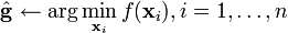While not converged:
- For each particle :
  - Create random vectors $\mathbf{r}_{1}$ , $\mathbf{r}_{2}$ : $\mathbf{r}_{1 j}$ and $\mathbf{r}_{2 j}$ for all $j$ ,by taking $\mathbf{r}_{1 j},\mathbf{r}_{2 j} \in U[0, 1]$ for $j = 1, \ldots, m$
  - Update the particle positions: $\mathbf{x}_i \leftarrow \mathbf{x}_i+\mathbf{v}_i$ .
  - Update the particle velocities: $\mathbf{v}_i \leftarrow {\omega}\mathbf{v}_i+c_1\mathbf{r}_1\circ(\hat{\mathbf{x}}_i-\mathbf{x}_i)+c_2\mathbf{r}_2\circ(\hat{\mathbf{g}}-\mathbf{x}_i)$ .
  - Update the local bests: If $f(\mathbf{x}_i) < f(\hat{\mathbf{x}}_i)$ , $\hat{\mathbf{x}}_i \leftarrow \mathbf{x}_i$ .
  - Update the global best If $f(\mathbf{x}_i) < f(\hat{\mathbf{g}})$ , $\hat{\mathbf{g}} \leftarrow \mathbf{x}_i$ .
$\hat{\mathbf{g}}$ is the optimal solution with fitness $f(\hat{\mathbf{g}})$ .

Note the following about the above algorithm:

$ω$ is an inertial constant. Good values are usually slightly less than 1.
$c 1$ and $c 2$ are constants that say how much the particle is directed towards good positions. They represent a "cognitive" and a "social" component, respectively, in that they affect how much the particle's personal best and the global best (respectively) influence its movement. Usually we take $c_1, c_2 \approx 2$ .
$\mathbf{r}_1, \mathbf{r}_2$ are two random vectors with each component generally a uniform random number between 0 and 1.
$\circ$ operator indicates element-by-element multiplication i.e. the Hadamard matrix multiplication operator.

- - Note that there is a misconception arising from the tendency to write the velocity formula in a "vector notation" (see for example D.N. Wilke's papers). The original intent (see M.C.'s "Particle Swarm Optimization, 2006") was to multiply a NEW random component per dimension, rather than multiplying the same component with each dimension per particle. Moreover, r1 and r2 are supposed to consist of a single number, defined as Cmax, which normally has a relationship with omega (defined as C1 in the literature) through a transcendental function, given the value 'phi': C1 = 1.0 / (phi - 1.0 + (v_phi * v_phi) - (2.0 * v_phi)) - and - Cmax = C1 * phi. Optimal "confidence coefficients" are therefore approximately in the ratio scale of C1=0.7 and Cmax=1.43. The Pseudo code shown below however, describes the intent correctly - mishka

[edit] Pseudo code

Here follows a pseudo code example of the basic PSO. Note that the random vectors $\mathbf{r}_1, \mathbf{r}_2$ are implemented as scalars inside the dimension loop which is equivalent to the mathematical description given above.

 // Initialize the particle positions and their velocities
 for I = 1 to number of particles n do
   for J = 1 to number of dimensions m do
      X[I][J] = lower limit + (upper limit - lower limit) * uniform random number 
      V[I][J] = 0
   enddo
 enddo
 
 // Initialize the global and local fitness to the worst possible
 fitness_gbest = inf;
 for I = 1 to number of particles n do
    fitness_lbest[I] = inf
 enddo
 
 // Loop until convergence, in this example a finite number of iterations chosen
 for k = 1 to number of iterations t do
   
   // evaluate the fitness of each particle
   fitness_X = evaluate_fitness(X)
   
   // Update the local bests and their fitness 
   for I = 1 to number of particles n do
     if (fitness_X[I] < fitness_lbest[I])
       fitness_lbest[I] = fitness_X[I]
       for J = 1 to number of dimensions m do
         X_lbest[I][J] = X[I][J]
       enddo
     endif
   enddo
   
   // Update the global best and its fitness 
   [min_fitness, min_fitness_index] = min(fitness_X)
   if (min_fitness < fitness_gbest)
       fitness_gbest = min_fitness
       for J = 1 to number of dimensions m do
         X_gbest[J] = X(min_fitness_index,J)
       enddo
   endif
   
   // Update the particle velocity and position
   for I = 1 to number of particles n do
     for J = 1 to number of dimensions m do
       R1 = uniform random number
       R2 = uniform random number
       V[I][J] = w*V[I][J]
              + C1*R1*(X_lbest[I][J] - X[I][J])
              + C2*R2*(X_gbest[J] - X[I][J])
       X[I][J] = X[I][J] + V[I][J]
     enddo
   enddo
   
 enddo

[edit] Discussion

By studying this algorithm, we see that we are essentially carrying out something like a discrete-time simulation where each iteration of it represents a tick of time. The particles communicate information they find about each other by updating their velocities in terms of local and global bests. When a new best is found, the particles will change their positions accordingly so that the new information is broadcast to the swarm. The particles are always drawn back both to their own personal best positions and also to the best position of the entire swarm. They also have stochastic exploration capability via the use of the random multipliers $r 1, r 2$ . The vector, floating-point nature of the algorithm suggests that high-performance implementations could be created that take advantage of modern hardware extensions pertaining to vectorization, such as Streaming SIMD Extensions and Altivec.

Typical convergence conditions include reaching a certain number of iterations, reaching a certain fitness value, and so on.

[edit] Variations and practicalities

There are a number of considerations in using PSO in practice; one might wish to clamp the velocities to a certain maximum amount, for instance. The considerable adaptability of PSO to variations and hybrids is seen as a strength over other robust evolutionary optimization mechanisms, such as genetic algorithms. For example, one common, reasonable modification is to add a probabilistic bit-flipping local search heuristic to the loop. Normally, a stochastic hill-climber risks getting stuck at local maxima, but the stochastic exploration and communication of the swarm overcomes this. Thus, PSO can be seen as a basic search "workbench" that can be adapted as needed for the problem at hand.

Note that the research literature has uncovered many heuristics and variants determined to be better with respect to convergence speed and robustness, such as clever choices of $ω$ , $c i$ , and $r i$ . There are also other variants of the algorithm, such as discretized versions for searching over subsets of $\mathbb{Z}^n$ rather than $\mathbb{R}^n$ . There has also been experimentation with coevolutionary versions of the PSO algorithm with good results reported. Very frequently the value of $ω$ is taken to decrease over time; e.g., one might have the PSO run for a certain number of iterations and DECREASE linearly from a starting value (0.9, say) to a final value (0.4, say) in order to facilitate exploitation over exploration in later states of the search. The literature is full of such heuristics. In other words, the canonical PSO algorithm is not as strong as various improvements which have been developed on several common function optimization benchmarks and consulting the literature for ideas on parameter choices and variants for particular problems is likely to be helpful.

Significant, non-trivial modifications have been developed for multi-objective optimization, versions designed to find solutions satisfying linear or non-linear constraints, as well as "niching" versions designed to find multiple solutions to problems where it is believed or known that there are multiple global minima which ought to be located.

There is also a modified version of the algorithm called repulsive particle swarm optimization, in which a new factor, called repulsion, is added to the basic algorithm step.

[edit] Applications

Although a relatively new paradigm, PSO has been applied to a variety of tasks, such as the training of artificial neural networks and for finite element updating. Very recently, PSO has been applied in combination with grammatical evolution to create a hybrid optimization paradigm called "grammatical swarms".

[edit] See also

[edit] References

J. Kennedy and R. C. Eberhart. Swarm Intelligence. Morgan Kaufmann. 2001

M. Clerc. Particle Swarm Optimization. ISTE, 2006.

D. N. Wilke, S. Kok, and A. A. Groenwold, Comparison of linear and classical velocity update rules in particle swarm optimization: notes on diversity, International Journal for Numerical Methods in Engineering, Vol. 70, No. 8, pp. 962–984, 2007.

A. Chatterjee, P. Siarry, Nonlinear inertia variation for dynamic adaptation in particle swarm optimization, Computers and Operations Research, Vol. 33, No. 3, pp. 859–871, 2006.

A. P. Engelbrecht. Fundamentals of Computational Swarm Intelligence. Wiley, 2005. [1]

D. N. Wilke. Analysis of the particle swarm optimization algorithm, Master's Dissertation, University of Pretoria, 2005. [2]

T. Marwala. Finite element model updating using particle swarm optimization. International Journal of Engineering Simulation, 2005, 6(2), pp. 25-30. ISSN: 1468-1137.

M. Clerc, and J. Kennedy, The Particle Swarm-Explosion, Stability, and Convergence in a Multidimensional Complex Space, IEEE Transactions on Evolutionary Computation, 2002, 6, 58-73