Quantum electrodynamics

	Quantum field theory
	Feynman diagram
Background
	Gauge theory; Field theory; Poincaré symmetry; Quantum mechanics; Spontaneous symmetry breaking;
Symmetries
	Crossing; Charge conjugation; Parity; Time reversal;
Tools
	Anomaly; Effective field theory; Expectation value; Faddeev–Popov ghosts; Feynman diagram; LSZ reduction formula; Partition function; Propagator; Quantization; Renormalization; Vacuum state; Wick's theorem; Wightman axioms;
Equations
	Dirac equation; Klein–Gordon equation; Proca equations; Wheeler–deWitt equation;
Standard model
	Electroweak interaction; Higgs mechanism; Quantum chromodynamics; Quantum electrodynamics; Yang–Mills theory;
Incomplete theories
	Quantum gravity; String theory; Supersymmetry; Theory of everything
Scientists
	Adler • Bethe • Bogoliubov , Callan • Coleman • DeWitt • Dirac • Dyson • Fermi • Feynman • Fierz • Fröhlich • Gell-Mann • Goldstone • Gross • 't Hooft • Jackiw • Klein • Landau • Lee • Lehmann • Majorana • Nambu • Parisi • Polyakov • Salam • Schwinger • Skyrme • Stueckelberg •Symanzik • Tomonaga • Veltman • Weinberg • Weisskopf • Wilson • Witten • Yang • Yukawa • Zimmermann • Zinn-Justin
	This box: view • talk • edit

From Wikipedia, the free encyclopedia

Jump to: navigation, search

Quantum electrodynamics (QED) is a relativistic quantum field theory of electrodynamics. QED was developed by a number of physicists, beginning in the late 1920s. It basically describes how light and matter interact. More specifically it deals with the interactions between electrons, positrons and photons. QED mathematically describes all phenomena involving electrically charged particles interacting by means of exchange of photons. It has been called "the jewel of physics" for its extremely accurate predictions of quantities like the anomalous magnetic moment of the electron, and the Lamb shift of the energy levels of hydrogen.^[1]

In technical terms, QED can be described as a perturbation theory of the electromagnetic quantum vacuum.

[edit] History

Main article: History of quantum mechanics

The word 'quantum' is Latin, meaning "how much" (neut. sing. of quantus "how great").^[2] The word 'electrodynamics' was coined by André-Marie Ampère in 1822.^[3] The word 'quantum', as used in physics, i.e. with reference to the notion of count, was first used by Max Planck, in 1900 and reinforced by Einstein in 1905 with his use of the term light quanta.

Quantum theory began in 1900, when Max Planck assumed that energy is quantized in order to derive a formula predicting the observed frequency dependence of the energy emitted by a black body. This dependence is completely at variance with classical physics. In 1905, Einstein explained the photoelectric effect by postulating that light energy comes in quanta later called photons. In 1913, Bohr invoked quantization in his proposed explanation of the spectral lines of the hydrogen atom. In 1924, Louis de Broglie proposed a quantum theory of the wave-like nature of subatomic particles. The phrase "quantum physics" was first employed in Johnston's Planck's Universe in Light of Modern Physics. These theories, while they fit the experimental facts to some extent, were strictly phenomenological: they provided no rigorous justification for the quantization they employed.

Modern quantum mechanics was born in 1925 with Werner Heisenberg's matrix mechanics and Erwin Schrödinger's wave mechanics and the Schrödinger equation, which was a non-relativistic generalization of de Broglie's(1925) relativistic approach. Schrödinger subsequently showed that these two approaches were equivalent. In 1927, Heisenberg formulated his uncertainty principle, and the Copenhagen interpretation of quantum mechanics began to take shape. Around this time, Paul Dirac, in work culminating in his 1930 monograph finally joined quantum mechanics and special relativity, pioneered the use of operator theory, and devised the bra-ket notation widely used since. In 1932, John von Neumann formulated the rigorous mathematical basis for quantum mechanics as the theory of linear operators on Hilbert spaces. This and other work from the founding period remains valid and widely used.

Quantum chemistry began with Walter Heitler and Fritz London's 1927 quantum account of the covalent bond of the hydrogen molecule. Linus Pauling and others contributed to the subsequent development of quantum chemistry.

The application of quantum mechanics to fields rather than single particles, resulting in what are known as quantum field theories, began in 1927. Early contributors included Dirac, Wolfgang Pauli, Weisskopf, and Jordan. This line of research culminated in the 1940s in the quantum electrodynamics (QED) of Richard Feynman, Freeman Dyson, Julian Schwinger, and Sin-Itiro Tomonaga, for which Feynman, Schwinger and Tomonaga received the 1965 Nobel Prize in Physics. QED, a quantum theory of electrons, positrons, and the electromagnetic field, was the first satisfactory quantum description of a physical field and of the creation and annihilation of quantum particles.

QED involves a covariant and gauge invariant prescription for the calculation of observable quantities. Feynman's mathematical technique, based on his diagrams, initially seemed very different from the field-theoretic, operator-based approach of Schwinger and Tomonaga, but Freeman Dyson later showed that the two approaches were equivalent. The renormalization procedure for eliminating the awkward infinite predictions of quantum field theory was first implemented in QED. Even though renormalization works very well in practice, Feynman was never entirely comfortable with its mathematical validity, even referring to renormalization as a "shell game" and "hocus pocus". (Feynman, 1985: 128)

QED has served as the model and template for all subsequent quantum field theories. One such subsequent theory is quantum chromodynamics, which began in the early 1960s and attained its present form in the 1975 work by H. David Politzer, Sidney Coleman, David Gross and Frank Wilczek. Building on the pioneering work of Schwinger, Peter Higgs, Goldstone, and others, Sheldon Glashow, Steven Weinberg and Abdus Salam independently showed how the weak nuclear force and quantum electrodynamics could be merged into a single electroweak force.

[edit] Physical interpretation of QED

In classical optics, light travels over all allowed paths and their interference results in Fermat's principle. Similarly, in QED, light (or any other particle like an electron or a proton) passes over every possible path allowed by apertures or lenses. The observer (at a particular location) simply detects the mathematical result of all wave functions added up, as a sum of all line integrals. For other interpretations, paths are viewed as non physical, mathematical constructs that are equivalent to other, possibly infinite, sets of mathematical expansions. According to QED, light^{[dubious – discuss]} can go slower or faster than c, but will travel at velocity c on average^[4].

Physically, QED describes charged particles (and their antiparticles) interacting with each other by the exchange of photons. The magnitude of these interactions can be computed using perturbation theory; these rather complex formulas have a remarkable pictorial representation as Feynman diagrams. QED was the theory to which Feynman diagrams were first applied. These diagrams were invented on the basis of Lagrangian mechanics. Using a Feynman diagram, one decides every possible path between the start and end points. Each path is assigned a complex-valued probability amplitude, and the actual amplitude we observe is the sum of all amplitudes over all possible paths. The paths with stationary phase contribute most (due to lack of destructive interference with some neighboring counter-phase paths) — this results in the stationary classical path between the two points.

QED doesn't predict what will happen in an experiment, but it can predict the probability of what will happen in an experiment, which is how (statistically)it is experimentally verified. Predictions of QED agree with experiments to an extremely high degree of accuracy: currently about 10⁻¹² (and limited by experimental errors); for details see precision tests of QED. This makes QED one of the most accurate physical theories constructed thus far.

Near the end of his life, Richard P. Feynman gave a series of lectures on QED intended for the lay public. These lectures were transcribed and published as Feynman (1985), QED: The strange theory of light and matter, a classic non-mathematical exposition of QED from the point of view articulated above.

[edit] Mathematics

Mathematically, QED is an abelian gauge theory with the symmetry group U(1). The gauge field, which mediates the interaction between the charged spin-1/2 fields, is the electromagnetic field. The QED Lagrangian for a spin-1/2 field interacting with the electromagnetic field is given by the real part of

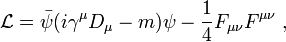
$\mathcal{L}=\bar\psi(i\gamma^\mu D_\mu-m)\psi -\frac{1}{4}F_{\mu\nu}F^{\mu\nu}\;,$

where

$\gamma_\mu \,\!$ are Dirac matrices;

$\ \psi$ a bispinor field of spin-1/2 particles (e.g. electron-positron field);

$\bar\psi\equiv\psi^\dagger\gamma_0$ , called "psi-bar", is sometimes referred to as Dirac adjoint;

$D_\mu = \partial_\mu+ieA_\mu+ieB_\mu \,\!$ is the gauge covariant derivative;

$\ e$ is the coupling constant, equal to the electric charge of the bispinor field;

$\ A_\mu$ is the covariant four-potential of the electromagnetic field generated by electron itself;

$\ B_\mu$ is the external field imposed by external source;

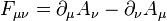$F_{\mu\nu} = \partial_\mu A_\nu - \partial_\nu A_\mu \,\!$ is the electromagnetic field tensor.

[edit] Euler-Lagrange equations

To begin, substituting the definition of D into the Lagrangian gives us:

$\mathcal{L} = i \bar{\psi} \gamma^\mu \partial_\mu \psi - e\bar{\psi}\gamma_\mu (A^\mu+B^\mu) \psi -m \bar{\psi} \psi - \frac{1}{4}F_{\mu\nu}F^{\mu\nu}. \quad \quad \,$

Next, we can substitute this Lagrangian into the Euler-Lagrange equation of motion for a field:

$\partial_\mu \left( \frac{\partial \mathcal{L}}{\partial ( \partial_\mu \psi )} \right) - \frac{\partial \mathcal{L}}{\partial \psi} = 0 \quad \quad \quad \quad \quad (2) \,$

to find the field equations for QED.

The two terms from this Lagrangian are then:

$\partial_\mu \left( \frac{\partial \mathcal{L}}{\partial ( \partial_\mu \psi )} \right) = \partial_\mu \left( i \bar{\psi} \gamma^\mu \right) \,$

$\frac{\partial \mathcal{L}}{\partial \psi} = -e\bar{\psi}\gamma_\mu (A^\mu+B^\mu) - m \bar{\psi}. \,$

Substituting these two back into the Euler-Lagrange equation (2) results in:

$i \partial_\mu \bar{\psi} \gamma^\mu + e\bar{\psi}\gamma_\mu (A^\mu+B^\mu) + m \bar{\psi} = 0 \,$

with complex conjugate:

$i \gamma^\mu \partial_\mu \psi - e \gamma_\mu (A^\mu+B^\mu) \psi - m \psi = 0. \,$

Bringing the middle term to the right-hand side transforms this second equation into:

$i \gamma^\mu \partial_\mu \psi - m \psi = e \gamma_\mu (A^\mu+B^\mu) \psi. \,$

The left-hand side is like the original Dirac equation and the right-hand side is the interaction with the electromagnetic field.

One further important equation can be found by substituting the Lagrangian into another Euler-Lagrange equation, this time for the field, $A μ$ :

$\partial_\nu \left( \frac{\partial \mathcal{L}}{\partial ( \partial_\nu A_\mu )} \right) - \frac{\partial \mathcal{L}}{\partial A_\mu} = 0 . \quad \quad \quad (3) \,$

The two terms this time are:

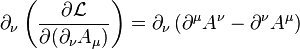
$\partial_\nu \left( \frac{\partial \mathcal{L}}{\partial ( \partial_\nu A_\mu )} \right) = \partial_\nu \left( \partial^\mu A^\nu - \partial^\nu A^\mu \right) \,$

$\frac{\partial \mathcal{L}}{\partial A_\mu} = -e\bar{\psi} \gamma^\mu \psi \,$

and these two terms, when substituted back into (3) give us:

$\partial_\nu F^{\nu \mu} = e \bar{\psi} \gamma^\mu \psi. \,$

Using perturbation theory, we could divide result into different parts according to the order of electric charge $q\,$ :

$\psi=\psi_0 + q \psi_1 + q^2 \psi_2 + o(q^3) \,$

here we use $q\,$ instead of $e\,$ to avoid confusion between electric charge $e\,$ and natural logarithm $e\,$

The zeroth order result is:

$\psi_0 (t, \vec{p})=e^{ \mp it \sqrt{p^2+m^2}} ( \dfrac{1}{2} \pm \dfrac{\vec{\alpha} \cdot \vec{p} +\beta m}{2\sqrt{p^2+m^2}}) \psi (0, \vec{p}) \,$

$\psi (t, \vec{p})$ is the 3-dimension momentum space expression of wave function:

$\psi (t, \vec{p})=(2 \pi)^{- \dfrac{3}{2}} \int \psi (t, \vec{x}) e^{-i \vec{x} \cdot \vec{p} } d \vec{x} \,$

The 1st order result (ignore the self energy $A^\mu \,$ )is:

$\psi_1 (t, \vec{p}) = (2 \pi)^{-2} \int [ \sum_{a_1,a_2=\pm 1} (\dfrac{1}{2} + \dfrac{\vec{\alpha} \cdot \vec{p} + \beta m}{2a_1 \sqrt{p^2+m^2}}) B^\mu (E,\vec{\tau}) \gamma_0 \gamma_\mu (\dfrac{1}{2} + \dfrac{\vec{\alpha} \cdot (\vec{p}-\vec{\tau}) + \beta m}{2a_2 \sqrt{p^2+m^2}}) \psi (0,\vec{p}-\vec{\tau}) (\dfrac{e^{-it a_1 \sqrt{p^2+m^2}}-1}{a_1 \sqrt{p^2+m^2}-E-a_2 \sqrt{(\vec{p}-\vec{\tau})^2+m^2})}+\dfrac{e^{-it(E+a_2\sqrt{(\vec{p}-\vec{\tau})^2+m^2})}-1}{E+a_2\sqrt{(\vec{p}-\vec{\tau})^2+m^2}-a_1 \sqrt{p^2+m^2}}) ] dE d \vec{\tau} \,$

The term $B^\mu (E,\vec{\tau})$ is the external field in 4-dimension momentum space:

$B^\mu (E,\vec{p}) =(2\pi)^{-2} \int B^\mu (t,\vec{x}) e^{i(Et-\vec{p}\cdot\vec{x})}dtd\vec{x}$

The solution of $A^{\mu} \,$ can be achieved in the same way(using Lorentz gauge $\partial_{\mu} A^{\mu}=0 \,$ ):

$A^{\mu}=A^{\mu}_0+eA^{\mu}_1+e^2 A^{\mu}_2 +o(e^3) \,$

$A^{\mu}_0=[A^{\mu}(0,\vec{p}) \pm \dfrac{1}{2p} i\dfrac{\partial A^{\mu}(t,\vec{p})}{\partial t}\mid _{t=0}]e^{\mp itp}$

$A^{\mu}_1=-(2 \pi)^{-\dfrac{3}{2}} \sum_{a_1,a_2,a_3=\pm 1} \dfrac{a_1}{2p} \int \psi^{\dagger}(0,\vec{\tau}) (\dfrac{1}{2} + \dfrac{\vec{\alpha} \cdot \vec{\tau} - \beta m}{2a_2 \sqrt{\tau^2+m^2}}) \gamma^0 \gamma^{\mu} (\dfrac{1}{2} + \dfrac{\vec{\alpha} \cdot (\vec{p}-\vec{\tau}) + \beta m}{2a_3 \sqrt{(\vec{p}-\vec{\tau})^2+m^2}}) \psi (0,\vec{p}-\vec{\tau}) (\dfrac{e^{-itb_1}-1}{b_1-b_2}+\dfrac{e^{-itb_2}-1}{b_2-b_1} ) d\vec{\tau} \,$

in which:

$b_1=a_1 p\,$

$b_2=a_2 \sqrt{\tau^2+m^2}+a_3 \sqrt{(\vec{p}-\vec{\tau})^2 +m^2 } \,$

[edit] In pictures

The part of the Lagrangian containing the electromagnetic field tensor describes the free evolution of the electromagnetic field, whereas the Dirac-like equation with the gauge covariant derivative describes the free evolution of the electron and positron fields as well as their interaction with the electromagnetic field.

The one-loop contribution to the vacuum polarization function $\Pi\,$

The one-loop contribution to the electron self-energy function $\Sigma \,$

The one-loop contribution to the vertex function $\Gamma\,$

[edit] See also

Physics portal

[edit] References

^ Feynman, Richard (1985). "Chapter 1". QED: The Strange Theory of Light and Matter. Princeton University Press. p. 6. http://www.amazon.com/gp/reader/0691024170.
^ Online Etymology Dictionary
^ Grandy, W.T. (2001). Relativistic Quantum Mechanics of Leptons and Fields, Springer.
^ Richard P. Feynman QED:(QED (book)) p89-90 "the light has an amplitude to go faster or slower than the speed c, but these amplitudes cancel each other out over long distances"; see also accompanying text

[edit] Further reading

[edit] Books

Feynman, Richard Phillips (1998). Quantum Electrodynamics. Westview Press; New Ed edition. ISBN 978-0201360752.
Tannoudji-Cohen, Claude; Dupont-Roc, Jacques, and Grynberg, Gilbert (1997). Photons and Atoms: Introduction to Quantum Electrodynamics. Wiley-Interscience. ISBN 978-0471184331.
De Broglie, Louis (1925). Recherches sur la theorie des quanta [Research on quantum theory]. France: Wiley-Interscience.
Jauch, J.M.; Rohrlich, F. (1980). The Theory of Photons and Electrons. Springer-Verlag. ISBN 978-0387072951.
Miller, Arthur I. (1995). Early Quantum Electrodynamics : A Sourcebook. Cambridge University Press. ISBN 978-0521568913.
Schweber, Silvian, S. (1994). QED and the Men Who Made It. Princeton University Press. ISBN 978-0691033273.
Schwinger, Julian (1958). Selected Papers on Quantum Electrodynamics. Dover Publications. ISBN 978-0486604442.
Greiner, Walter; Bromley, D.A.,Müller, Berndt. (2000). Gauge Theory of Weak Interactions. Springer. ISBN 978-3540676720.
Kane, Gordon, L. (1993). Modern Elementary Particle Physics. Westview Press. ISBN 978-0201624601.

[edit] Journals

J.M. Dudley and A.M. Kwan, "Richard Feynman's popular lectures on quantum electrodynamics: The 1979 Robb Lectures at Auckland University," American Journal of Physics Vol. 64 (June 1996) 694-698.

Challenged by Utan Skriboa, Nrahif Sansbah and Sarah Carpenter, Jacobs School of Engineering via University of California San Diego, (2003)

[edit] External links

[0] Feynman, Richard (1985). "Chapter 1". QED: The Strange Theory of Light and Matter. Princeton University Press. p. 6. http://www.amazon.com/gp/reader/0691024170.

[1] Online Etymology Dictionary

[2] Grandy, W.T. (2001). Relativistic Quantum Mechanics of Leptons and Fields, Springer.

[3] Richard P. Feynman QED:(QED (book)) p89-90 "the light has an amplitude to go faster or slower than the speed c, but these amplitudes cancel each other out over long distances"; see also accompanying text

[1]

[2]

[3]

[4]

Quantum electrodynamics

From Wikipedia, the free encyclopedia

Contents

[edit] History

[edit] Physical interpretation of QED

[edit] Mathematics

[edit] Euler-Lagrange equations

[edit] In pictures

[edit] See also

[edit] References

[edit] Further reading

[edit] Books

[edit] Journals

[edit] External links

Views

Personal tools

Navigation

Search

Interaction

Toolbox

Languages