Hasse diagram
From Wikipedia, the free encyclopedia
In the mathematical discipline known as order theory, a Hasse diagram (pronounced /ˈhɑːsə/ HAHS uh) is a simple picture of a finite partially ordered set, forming a drawing of the transitive reduction of the partial order. Concretely, for a partially ordered set (S, ≤) one represents each element of S as a vertex on the page and draws a line segment or curve that goes upward from x to y if x < y, and there is no z such that x < z < y (here, < is obtained from ≤ by removing elements (x,x) for all x). In this case, we say y covers x, or y is an immediate successor of x. Furthermore it is required that the vertices are positioned in such a way that each curve meets exactly two vertices: its two endpoints. Any such diagram (given that the vertices are labeled) uniquely determines a partial order, and any finite partial order has a unique transitive reduction,[1] but there are many possible placements of elements in the plane, resulting in different Hasse diagrams for a given order that may have widely varying appearances.
Hasse diagrams are named after Helmut Hasse (1898–1979); according to Birkhoff (1948), they are so-called because of the effective use Hasse made of them. However, Hasse was not the first to use these diagrams; they appear, e.g., in Vogt (1895). Although Hasse diagrams were originally devised as a technique for making drawings of partially ordered sets by hand, they have more recently been created automatically using graph drawing techniques.[2]
Sometimes, the phrase "Hasse diagram" is used to refer to the transitive reduction as an abstract directed acyclic graph, independently of any drawing of that graph, but this usage is eschewed here.
Contents |
[edit] Examples
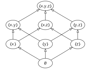
- The power set of { x, y, z } partially ordered by inclusion, has the Hasse diagram:
- The set A = { 1, 2, 3, 4, 5, 6, 10, 12, 15, 20, 30, 60 } of all divisors of 60, partially ordered by divisibility, has the Hasse diagram:

- The set of all 15 partitions of the set { 1, 2, 3, 4 }, partially ordered by "refinement", i.e. a finer partition is "less than" a coarser partition, has the Hasse diagram:

[edit] Cayley graph
A group and a set of generators determine two partial orders (the weak order and the Bruhat order), and correspondingly two Hasse diagrams. This is particularly applied to Coxeter groups. The length of an element (distance from the identity in the word metric, equivalently, shortest length of a reduced word) determines a length function.
In the weak order, an element h exceeds an element g if a reduced word for g is a prefix of a reduced word for h, and the Hasse diagram is obtained from the Cayley graph by deleting edges: only edges connecting an element of length k to an element of length k+1 are retained (i.e., edges that are part of the transitive reduction).
[edit] Motivation
If we were to try to create some visual representation of a partially ordered set (S, ≤), how would we proceed? We could begin by first creating a graph, where every node on the graph is an element in S, and every edge (u, v) in that graph would represent the relation u ≤ v.
Doing this, and trying to draw the graph, would result in a graph that would be very "busy". In fact, we carry a lot of redundant information in such a graph. Recall the requirements on a partial order:
- a ≤ a (reflexivity)
- if a ≤ b and b ≤ c then a ≤ c (transitivity)
- if a ≤ b and b ≤ a then a = b (antisymmetry)
Now, in our original graph, we have a number of edges — loops, on each node in the graph — in the form (u, u), because reflexivity means that u ≤ u. This must be true for every element in S (otherwise it would not be a partial order).
Say we were now to create a diagram, as above now, without loops, of the partially ordered set ({1,2,3,4}, ≤), where a finer partition of that set is "less than" a coarser partition. We would obtain the following graph:

However, in this graph, we still carry redundant information. Referring back to the requirements of a partial order, we see the requirement of transitivity. In the above graph, we are including edges (a,c), (a,b), and (b,c). We do not need to carry the extra edge (a,c) because the other two edges imply the third exists.
This means we need only include an edge between a member of the set, and its immediate predecessor. We do not need the edges to the other predecessors because we have transitivity, nor do we need to draw loops at each edge because we have reflexivity.
If we were to stop here and draw the diagram again according to these new requirements, we obtain the third image above, in the Example section. We can stop here, but it may be useful to define the Hasse diagram in terms of another relation which automatically excludes these cases.
[edit] Cover relation
Symbolically, all edges in the Hasse diagram should be of the form (x, y) where x < y (this stricter relation means we exclude cases of loops as before), and that there exists no element z in the set such that x < z < y (this is another way of excluding drawing extra edges because of transitivity).
This relation is known as the cover relation, and the Hasse diagram is often defined in terms of this relation. An element y is said to cover x if y is an immediate successor of x. The (strict) partial ordering is then just the transitive closure of this cover relation.
The Hasse diagram of S may then be defined abstractly as the set of all ordered pairs (x, y) such that y covers x, i.e., the Hasse diagram may be identified with the inverse of the cover relation.
[edit] Finding a "good" Hasse diagram
Although Hasse diagrams are simple as well as intuitive tools for dealing with finite posets, it turns out to be rather difficult to draw "good" diagrams. The reason is that there are in general many (in fact: infinitely many) possible ways to draw a Hasse diagram for a given poset. The simple technique of just starting with the minimal elements of an order and then adding greater elements incrementally often produces quite poor results: symmetries and internal structure of the order are easily lost.
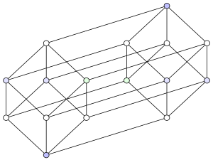
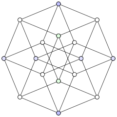
The following example demonstrates the problem. Consider the powerset of the set S = {a, b, c, d}, i.e. the set of all subsets of S, written as  . This powerset can easily be ordered via subset inclusion
  . Below there are three different principal ways to draw a Hasse diagram for this order:
 |
 |
 |
 |
The leftmost version, respectively the big diagram below, is probably closest to the naive way of constructing diagrams: the five layers of the graph represent the numbers of elements that the subsets at each level contain. Note that there are many different ways to assign concrete one-element sets to the second layer, but that this assignment will determine the labels of all other elements. The circumstance that more than one labeling of each of the diagrams is possible reflects the fact that the poset in this example is automorphic — even in many different ways. (If nothing speaks against it, it is recommendable to use the lexicographical order for the first layer.)
The above example demonstrates how different Hasse diagrams for the same order can be, and how each representation can reflect different aspects of the underlying mathematical structure. The leftmost diagram relates the number of elements to the level of each vertex. The rightmost drawing strongly emphasizes the internal symmetry of the structure. Finally, the middle one constructs the picture from two cubes such that the relationship between the powerset 2S and the product order 2 × 2{a, b, c} is emphasized.
Various algorithms for drawing better diagrams have been proposed, but today good diagrams still heavily rely on human assistance. However, even humans need quite some practice to draw instructive diagrams.
[edit] Polytopes
Hasse diagrams are very useful for illustrating the combinatorial structure of polytopes – the hierarchy of their vertices, edges, faces etc. In abstract polytope theory, the Hasse diagram (or more precisely, the poset) is the polytope.
[edit] See also
[edit] Notes
- ^ Infinite partial orders need not have a transitive reduction, as elements need to have immediate successors: consider the real interval [0,1].
- ^ E.g., see Di Battista & Tamassia (1988) and Freese (2004).
[edit] References
- Birkhoff, Garrett (1948), Lattice Theory (Revised ed.), American Mathematical Society.
- Di Battista, G.; Tamassia, R. (1988), "Algorithms for plane representation of acyclic digraphs", Theoretical Computer Science 61: 175–178.
- Freese, Ralph (2004), "Automated lattice drawing", Concept Lattices, Lecture Notes in Computer Science, 2961, Springer-Verlag, pp. 589–590. An extended preprint is available online: [1].
- Vogt, Henri Gustav (1895), Leçons sur la résolution algébrique des équations, Nony, p. 91.
[edit] External links
| Wikimedia Commons has media related to: Hasse diagrams |

