Likelihood function

From Wikipedia, the free encyclopedia

In statistics, the likelihood function (often simply the likelihood) is a function of the parameters of a statistical model that plays a key role in statistical inference. In non-technical usage, "likelihood" is a synonym for "probability", but throughout this article only the technical definition is used. Informally, if "probability" allows us to predict unknown outcomes based on known parameters, then "likelihood" allows us to estimate unknown parameters based on known outcomes.

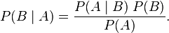
In a sense, likelihood works backwards from probability: given parameter B, we use the conditional probability P(A|B) to reason about outcome A, and given outcome A, we use the likelihood function L(B|A) to reason about parameter B. This mode of reasoning is formalized in Bayes' theorem:

$P(B \mid A) = \frac{P(A \mid B)\;P(B)}{P(A)}.\!$

A likelihood function is a conditional probability function considered as a function of its second argument with its first argument held fixed, thus:

$b\mapsto P(A \mid B=b), \!$

and also any other function proportional to such a function. That is, the likelihood function for B is the equivalence class of functions

$L(b \mid A) = \alpha \; P(A \mid B=b) \!$

for any constant of proportionality $α > 0$ . The numerical value $L (b | A)$ alone is immaterial; all that matters are likelihood ratios of the form

$\frac{L(b_2 | A)}{L(b_1 | A)}, \!$

which are invariant with respect to the constant of proportionality.

A. W. F. Edwards defined support as the natural logarithm of the likelihood ratio, and the support function as the natural logarithm of the likelihood function.^[1] There is potential for confusion with the mathematical meaning of 'support', however, and this terminology is not widely used outside Edwards' main applied field of phylogenetics.

For more about making inferences via likelihood functions, see also the method of maximum likelihood, and likelihood-ratio testing.

[edit] Likelihood function of a parameterized model

Among many applications, we consider here one of broad theoretical and practical importance. Given a parameterized family of probability density functions (or probability mass functions in the case of discrete distributions)

$x\mapsto f(x\mid\theta), \!$

where θ is the parameter, the likelihood function is

$\theta\mapsto f(x\mid\theta), \!$

written

$L(\theta \mid x)=f(x\mid\theta), \!$

where x is the observed outcome of an experiment. In other words, when f(x | θ) is viewed as a function of x with θ fixed, it is a probability density function, and when viewed as a function of θ with x fixed, it is a likelihood function.

Note: This is not the same as the probability that those parameters are the right ones, given the observed sample. Attempting to interpret the likelihood of a hypothesis given observed evidence as the probability of the hypothesis is a common error, with potentially disastrous real-world consequences in medicine, engineering or jurisprudence. See prosecutor's fallacy for an example of this.

From a geometric standpoint, If we consider f (x,θ) as a function of two variables, then the family of probability distributions can be viewed as level curves parallel to the θ -axis, while the family of likelihood functions are the orthogonal level curves parallel to the x-axis.

[edit] Likelihoods for continuous distributions

The use of the probability density instead of a probability in specifying the likelihood function above may be justified in a simple way. Suppose that, instead of an exact observation, x, the observation is the value in a short interval (x_j-1,x_j), with length Δ_j, where the subscripts refer to a predefined set of intervals. Then the probability of getting this observation (of being in interval j) is approximately

$L_\text{approx}(\theta \mid x \text{ in interval } j)=\Delta_j f(x_{*}\mid\theta), \!$

where x_* can be any point in interval j. Then, recalling that the likelihood function is defined up to a multiplicative constant, it is just as valid to say that the likelihood function is approximately

$L_\text{approx}(\theta \mid x \text{ in interval } j)= f(x_{*}\mid\theta), \!$

and then, on considering the lengths of the intervals to decrease to zero,

$L(\theta \mid x )= f(x\mid\theta). \!$

[edit] Likelihoods for mixed continuous — discrete distributions

The above can be extended in a simple way to allow consideration of distributions which contain both discrete and continuous components. Suppose that the distribution consists of a number of discrete probability masses p_k(θ) and a density f(x|θ), where the sum of all the p's added to the integral of f is always one. Assuming that it is possible to distinguish an observation corresponding to one of the discrete probability masses from one which corresponds to the density component, the likelihood function for an observation from the continuous component can be dealt with as above by setting the interval length short enough to exclude any of the discrete masses. For an observation from the discrete component, the probability can either be written down directly or treated within the above context by saying that the probability of getting an observation in an interval that does contain a discrete component (of being in interval j which contains discrete component k) is approximately

$L_\text{approx}(\theta \mid x \text{ in interval } j \text{ containing discrete mass } k)=p_k(\theta)+\Delta_j f(x_{*}\mid\theta), \!$

where x_* can be any point in interval j. Then, on considering the lengths of the intervals to decrease to zero, the likelihood function for a observation from the discrete component is

$L(\theta \mid x )= p_k(\theta), \!$

where k is the index of the discrete probability mass corresponding to observation x.

The fact that the likelihood function can be defined in a way that includes contributions that are not commensurate (the density and the probability mass) arises from the way in which the likelihood function is defined up to a constant of proportionality, where this "constant" can change with the observation x, but not with the parameter θ.

[edit] Example 1

The likelihood function for estimating the probability of a coin landing heads-up without prior knowledge after observing HH

The likelihood function for estimating the probability of a coin landing heads-up without prior knowledge after observing HHT

For example, a coin is tossed with a probability p_H of landing heads up ('H'), the probability of getting two heads in two trials ('HH') is p_H². If p_H = 0.5, then the probability of seeing two heads is 0.25.

In symbols, we can say the above as

$P(\mbox{HH} \mid p_H = 0.5) = 0.25$

Another way of saying this is to reverse it and say that "the likelihood of p_H = 0.5, given the observation 'HH', is 0.25", i.e.,

$L(p_H=0.5 \mid \mbox{HH}) = P(\mbox{HH}\mid p_H=0.5) =0.25$ .

But this is not the same as saying that the probability of p_H = 0.5, given the observation, is 0.25.

To take an extreme case, on this basis we can say "the likelihood of p_H = 1 given the observation 'HH' is 1". But it is clearly not the case that the probability of p_H = 1 given the observation is 1: the event 'HH' can occur for any p_H > 0 (and often does, in reality, for p_H roughly 0.5). If the probability of p_H = 1 given the observation is 1, it means that p_H must and can only be equal 1 for event 'HH' to occur which is obviously not true.

The likelihood function is not a probability density function – for example, the integral of a likelihood function is not in general 1. In this example, the integral of the likelihood over the interval [0, 1] in p_H is 1/3, demonstrating again that the likelihood function cannot be interpreted as a probability density function for p_H. On the other hand, given any particular value of p_H, e.g. p_H = 0.5, the integral of the probability density function over the domain of the random variables is 1.

[edit] Example 2

Main article: Maximum of a discrete uniform distribution

Consider a jar containing N lottery tickets numbered from 1 through N. If you pick a ticket randomly you get number n with probability 1/N if n ≤ N, and zero if n > N. This is written

$P(n|N)= \frac{[n \le N]}{N}$

where the Iverson bracket [n ≤ N] is 1 when n ≤ N and 0 otherwise. When considered a function of n for fixed N this is the probability distribution, but when considered a function of N for fixed n this is a likelihood function. The maximum likelihood estimate for N is N₀ = n (by contrast, the unbiased estimate is 2n − 1).

This likelihood function is not a probability distribution, because the total

$\sum_{N=1}^\infty P(n|N) = \sum_{N=1}^\infty \frac{[n \le N]}{N} = \sum_{N=n}^\infty \frac{1}{N}$

is a divergent series.

Suppose, however, that you pick two tickets rather than one.

The probability of the outcome {n₁, n₂}, where n₁ < n₂, is

$P(\{n_1,n_2\}|N)= \frac{[n_2 \le N]}{\binom N 2} .$

When considered a function of N for fixed n₂, this is a likelihood function. The maximum likelihood estimate for N is N₀ = n₂.

This time the total

$\sum_{N=1}^\infty P(\{n_1,n_2\}|N) = \sum_{N=1}^\infty \frac{[n_2 \le N]}{\binom N 2} = \sum_{N=n_2}^\infty \frac{1}{\binom N 2}$

is a convergent series, and so this likelihood function can be normalized into a probability distribution.

If you pick 3 or more tickets the likelihood function has a well defined mean value, which is larger than the maximum likelihood estimate. If you pick 4 or more tickets the likelihood function has a well defined standard deviation too.

[edit] Likelihoods that eliminate nuisance parameters

In many cases, the likelihood is a function of more than one parameter but interest focusses on the estimation of only one or at most a few of them, with the others being considered as nuisance parameters. Several alternative ways have been developed to eliminate such nuisance parameters so that a likelihood can be written as a function of the parameter (or parameters) of interest only, the main ones being marginal, conditional and profile likelihoods.^[2] ^[3]

These are useful because standard likelihood methods can become unreliable or fail entirely when there are many nuisance parameters (or the nuisance parameter is high-dimensional), particularly when the number of nuisance parameters is a substantial fraction of the number of observations and this fraction does not decrease when the sample size increases. They can also be used to derive closed-form formulae for statistical tests when direct use of maximum likelihood requires iterative numerical methods, and find application in some specialized topics such as sequential analysis.

[edit] Conditional likelihood

Sometimes it is possible to find a sufficient statistic for the nuisance parameters, and conditioning on this statistic results in a likelihood which does not depend on the nuisance parameters.

One example occurs in 2×2 tables, where conditioning on all four marginal totals leads to a conditional likelihood based on the non-central hypergeometric distribution. (This form of conditioning is also the basis for Fisher's exact test.)

[edit] Marginal likelihood

Main article: Marginal likelihood

Sometimes we can remove the nuisance parameters by considering a likelihood based on only part of the information in the data, for example by using the set of ranks rather than the numerical values. Another example occurs in linear mixed models, where considering a likelihood for the residuals only after fitting the fixed effects leads to residual maximum likelihood estimation of the variance components.

[edit] Profile likelihood

It is often possible to write some parameters as functions of other parameters, thereby reducing the number of independent parameters. (The function is the parameter value which maximises the likelihood given the value of the other parameters.) This procedure is called concentration of the parameters and results in the concentrated likelihood function, also occasionally known as the maximized likelihood function, but most often called the profile likelihood function.

For example, consider a regression analysis model with normally distributed errors. The most likely value of the error variance is the variance of the residuals. The residuals depend on all other parameters. Hence the variance parameter can be written as a function of the other parameters.

Unlike conditional and marginal likelihoods, profile likelihood methods can always be used (even when the profile likelihood cannot be written down explicitly). However, the profile likelihood is not a true likelihood as it is not based directly on a probability distribution and this leads to some less satisfactory properties. (Attempts have been made to improve this, resulting in modified profile likelihood.)

The idea of profile likelihood can also be used to compute confidence intervals that often have better small-sample properties than those based on asymptotic standard errors calculated from the full likelihood.

[edit] Partial likelihood

A partial likelihood is a factor component of the likelihood function that isolates the parameters of interest.^[4] It is a key component of the proportional hazards model.

[edit] Historical remarks

Some early thoughts on likelihood were made in a book by Thorvald N. Thiele published in 1889^[5]. The first paper where the full idea of the "likelihood" appears was written by R.A. Fisher in 1922^[6]: "On the mathematical foundations of theoretical statistics". In that paper, Fisher also uses the term "method of maximum likelihood". Fisher argues against inverse probability as a basis for statistical inferences, and instead proposes inferences based on likelihood functions.

[edit] See also

[edit] References

^ Edwards, A.W.F. 1972. Likelihood. Cambridge University Press, Cambridge (expanded edition, 1992, Johns Hopkins University Press, Baltimore). ISBN 0-8018-4443-6
^ Pawitan, Yudi (2001). In All Likelihood: Statistical Modelling and Inference Using Likelihood. Oxford University Press. ISBN 0198507658.
^ Wen Hsiang Wei. "Generalized linear model course notes". Tung Hai University, Taichung, Taiwan. Chapter 5. http://web.thu.edu.tw/wenwei/www/glmpdfmargin.htm. Retrieved on 2007-01-23.
^ Cox, D. R. (1975). "Partial likelihood". Biometrika 62 (2): 269–276. doi:10.1093/biomet/62.2.269. MR 0400509.
^ Steffen L. Lauritzen, Aspects of T. N. Thiele's Contributions to Statistics (1999).
^ Ronald A. Fisher. "On the mathematical foundations of theoretical statistics". Philosophical Transactions of the Royal Society, A, 222:309-368 (1922). ("Likelihood" is discussed in section 6.)

[edit] External links

Likelihood function at Planetmath

[0] Edwards, A.W.F. 1972. Likelihood. Cambridge University Press, Cambridge (expanded edition, 1992, Johns Hopkins University Press, Baltimore). ISBN 0-8018-4443-6

[1] Pawitan, Yudi (2001). In All Likelihood: Statistical Modelling and Inference Using Likelihood. Oxford University Press. ISBN 0198507658.

[2] Wen Hsiang Wei. "Generalized linear model course notes". Tung Hai University, Taichung, Taiwan. Chapter 5. http://web.thu.edu.tw/wenwei/www/glmpdfmargin.htm. Retrieved on 2007-01-23.

[3] Cox, D. R. (1975). "Partial likelihood". Biometrika 62 (2): 269–276. doi:10.1093/biomet/62.2.269. MR 0400509.

[4] Steffen L. Lauritzen, Aspects of T. N. Thiele's Contributions to Statistics (1999).

[5] Ronald A. Fisher. "On the mathematical foundations of theoretical statistics". Philosophical Transactions of the Royal Society, A, 222:309-368 (1922). ("Likelihood" is discussed in section 6.)

[1]

[2]

[3]

[4]

[5]

[6]

Likelihood function

From Wikipedia, the free encyclopedia

Contents

[edit] Likelihood function of a parameterized model

[edit] Likelihoods for continuous distributions

[edit] Likelihoods for mixed continuous — discrete distributions

[edit] Example 1

[edit] Example 2

[edit] Likelihoods that eliminate nuisance parameters

[edit] Conditional likelihood

[edit] Marginal likelihood

[edit] Profile likelihood

[edit] Partial likelihood

[edit] Historical remarks

[edit] See also

[edit] References

[edit] External links

Views

Personal tools

Navigation

Search

Interaction

Toolbox

Languages