Brownian motion
From Wikipedia, the free encyclopedia
- This article is about the physical phenomenon; for the stochastic process, see Wiener process. For the sports team, see Brownian Motion (Ultimate). For the mobility model, see Random walk.


Brownian motion (named after the Scottish botanist Robert Brown) is the seemingly random movement of particles suspended in a fluid (i.e. a liquid or gas) or the mathematical model used to describe such random movements, often called a particle theory.
The mathematical model of Brownian motion has several real-world applications. An often quoted example is stock market fluctuations.
Brownian motion is among the simplest of the continuous-time stochastic (or random) processes, and it is a limit of both simpler and more complicated stochastic processes (see random walk and Donsker's theorem). This universality is closely related to the universality of the normal distribution. In both cases, it is often mathematical convenience rather than the accuracy of the models that motivates their use.[clarification needed]
Contents |
[edit] History

The Roman Lucretius's scientific poem On the Nature of Things (c. 60 BC) has a remarkable description of Brownian motion of dust particles. He uses this as a proof of the existence of atoms: "Observe what happens when sunbeams are admitted into a building and shed light on its shadowy places. You will see a multitude of tiny particles mingling in a multitude of ways... their dancing is an actual indication of underlying movements of matter that are hidden from our sight... It originates with the atoms which move of themselves [i.e. spontaneously]. Then those small compound bodies that are least removed from the impetus of the atoms are set in motion by the impact of their invisible blows and in turn cannon against slightly larger bodies. So the movement mounts up from the atoms and gradually emerges to the level of our senses, so that those bodies are in motion that we see in sunbeams, moved by blows that remain invisible." Although the mingling motion of dust particles is caused largely by air currents, the glittering, tumbling motion of small dust particles is indeed caused chiefly by true Brownian dynamics.
Jan Ingenhousz had described the irregular motion of coal dust particles on the surface of alcohol in 1785. Nevertheless Brownian motion is traditionally regarded as discovered by the botanist Robert Brown in 1827. It is believed that Brown was studying pollen particles floating in water under the microscope. He then observed minute particles within the vacuoles of the pollen grains executing a jittery motion. By repeating the experiment with particles of dust, he was able to rule out that the motion was due to pollen particles being 'alive', although the origin of the motion was yet to be explained.
The first person to describe the mathematics behind Brownian motion was Thorvald N. Thiele in 1880 in a paper on the method of least squares. This was followed independently by Louis Bachelier in 1900 in his PhD thesis "The theory of speculation", in which he presented a stochastic analysis of the stock and option markets. However, it was Albert Einstein's (in his 1905 paper) and Marian Smoluchowski's (1906) independent research of the problem that brought the solution to the attention of physicists, and presented it as a way to indirectly confirm the existence of atoms and molecules.
[edit] Intuitive metaphor
Consider a large balloon of 10 meters in diameter. Imagine this large balloon in a football stadium. The balloon is so large that it lies on top of many members of the crowd. Because they are excited, these fans hit the balloon at different times and in different directions with the motions being completely random. In the end, the balloon is pushed in random directions, so it should not move on average. Consider now the force exerted at a certain time. We might have 20 supporters pushing right, and 21 other supporters pushing left, where each supporter is exerting equivalent amounts of force. In this case, the forces exerted from the left side and the right side are imbalanced in favor of the left side; the balloon will move slightly to the left. This type of imbalance exists at all times, and it causes random motion of the balloon. If we look at this situation from far above, so that we cannot see the supporters, we see the large balloon as a small object animated by erratic movement.
Considering Brown's pollen particle moving randomly in water: we know that a water molecule is about 0.1 by 0.2 nm in size, whereas a pollen particle is roughly 25 µm in diameter, some 250,000 times larger. So the pollen particle may be likened to the balloon, and the water molecules to the fans except that in this case the balloon is surrounded by fans. The Brownian motion of a particle in a liquid is thus due to the instantaneous imbalance in the combined forces exerted by collisions of the particle with the much smaller liquid molecules (which are in random thermal motion) surrounding it.
An animation of the Brownian motion concept is available as a Java applet.
[edit] Modelling using differential equations
|
|
This article may be confusing or unclear to readers. Please help clarify the article; suggestions may be found on the talk page. (September 2007) |
The equations governing Brownian motion relate slightly differently to each of the two definitions of Brownian motion given at the start of this article.
[edit] Mathematical
for main article, see Wiener process.
In mathematics, the Wiener process is a continuous-time stochastic process named in honor of Norbert Wiener. It is one of the best known Lévy processes (càdlàg stochastic processes with stationary independent increments) and occurs frequently in pure and applied mathematics, economics and physics.
The Wiener process Wt is characterized by three facts:
- W0 = 0
- Wt is almost surely continuous
- Wt has independent increments with distribution
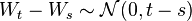 (for 0 ≤ s < t).
N(μ, σ2) denotes the normal distribution with expected value μ and variance σ2. The condition that it has independent increments means that if 0 ≤ s1 ≤ t1 ≤ s 2 ≤ t2 then Wt1 − Ws1 and Wt2 − Ws2 are independent random variables.
An alternative characterization of the Wiener process is the so-called Lévy characterization that says that the Wiener process is an almost surely continuous martingale with W0 = 0 and quadratic variation [Wt, Wt] = t.
A third characterization is that the Wiener process has a spectral representation as a sine series whose coefficients are independent N(0,1) random variables. This representation can be obtained using the Karhunen-Loève theorem.
The Wiener process can be constructed as the scaling limit of a random walk, or other discrete-time stochastic processes with stationary independent increments. This is known as Donsker's theorem. Like the random walk, the Wiener process is recurrent in one or two dimensions (meaning that it returns almost surely to any fixed neighborhood of the origin infinitely often) whereas it is not recurrent in dimensions three and higher. Unlike the random walk, it is scale invariant.
The time evolution of the position of the Brownian particle itself can be described approximately by a Langevin equation, an equation which involves a random force field representing the effect of the thermal fluctuations of the solvent on the Brownian particle. On long timescales, the mathematical Brownian motion is well described by a Langevin equation. On small timescales, inertial effects are prevalent in the Langevin equation. However the mathematical brownian motion is exempt of such inertial effects. Note that inertial effects have to be considered in the Langevin equation, otherwise the equation becomes singular, so that simply removing the inertia term from this equation would not yield an exact description, but rather a singular behavior in which the particle doesn't move at all.
[edit] Physical Brownian theory
The diffusion equation yields an approximation of the time evolution of the probability density function associated to the position of the particle undergoing a Brownian movement under the physical definition. The approximation is valid on short timescales (see Langevin equation for details).
The time evolution of the position of the Brownian particle itself is best described using Langevin equation, an equation which involves a random force field representing the effect of the thermal fluctuations of the solvent on the particle.
The displacement of a particle undergoing Brownian motion is obtained by solving the diffusion equation under appropriate boundary conditions and finding the rms of the solution. This shows that the displacement varies as the square root of the time (not linearly), which explains why previous experimental results concerning the velocity of Brownian particles gave nonsensical results. A linear time dependence was incorrectly assumed.
[edit] The Lévy characterization
The French mathematician Paul Lévy proved the following theorem, which gives a necessary and sufficient condition for a continuous Rn-valued stochastic process X to actually be n-dimensional Brownian motion. Hence, Lévy's condition can actually be used an alternative definition of Brownian motion.
Let X = (X1, ..., Xn) be a continuous stochastic process on a probability space (Ω, Σ, P) taking values in Rn. Then the following are equivalent:
- X is a Brownian motion with respect to P, i.e. the law of X with respect to P is the same as the law of an n-dimensional Brownian motion, i.e. the push-forward measure X∗(P) is classical Wiener measure on C0([0, +∞); Rn).
- both
- X is a martingale with respect to P (and its own natural filtration); and
- for all 1 ≤ i, j ≤ n, Xi(t)Xj(t) −δijt is a martingale with respect to P (and its own natural filtration), where δij denotes the Kronecker delta.
[edit] Brownian motion on a Riemannian manifold

The infinitesimal generator (and hence characteristic operator) of a Brownian motion on Rn is easily calculated to be ½Δ, where Δ denotes the Laplace operator. This observation is useful in defining Brownian motion on an m-dimensional Riemannian manifold (M, g): a Brownian motion on M is defined to be a diffusion on M whose characteristic operator  in local coordinates xi, 1 ≤ i ≤ m, is given by ½ΔLB, where ΔLB is the Laplace-Beltrami operator given in local coordinates by

where [gij] = [gij]−1 in the sense of the inverse of a square matrix.
[edit] See also
- Brownian bridge: a Brownian motion that is required to "bridge" specified values at specified times
- Brownian dynamics
- Brownian motor
- Brownian ratchet
- Brownian tree
- Rotational Brownian motion
- Complex system
- Diffusion equation
- Itō diffusion: a generalization of Brownian motion
- Langevin equation
- Local time (mathematics)
- Osmosis
- Red noise, also known as brown noise (Martin Gardner proposed this name for sound generated with random intervals. It is a pun on Brownian motion and white noise.)
- Schramm-Loewner evolution
- Surface diffusion - a type of constrained Brownian motion.
- Tyndall effect: physical chemistry phenomenon where particles are involved; used to differentiate between the different types of mixtures.
- Ultramicroscope
[edit] References
- Brown, Robert, "A brief account of microscopical observations made in the months of June, July and August, 1827, on the particles contained in the pollen of plants; and on the general existence of active molecules in organic and inorganic bodies." Phil. Mag. 4, 161-173, 1828. (PDF version of original paper including a subsequent defense by Brown of his original observations, Additional remarks on active molecules.)
- Einstein, A. (1905), "Über die von der molekularkinetischen Theorie der Wärme geforderte Bewegung von in ruhenden Flüssigkeiten suspendierten Teilchen.", Annalen der Physik 17: 549–560
- Smoluchowski, M. (1906), "Zur kinetischen Theorie der Brownschen Molekularbewegung und der Suspensionen", Annalen der Physik 21: 756–780
- Einstein, A. "Investigations on the Theory of Brownian Movement". New York: Dover, 1956. ISBN 0-486-60304-0 [1]
- Theile, T. N. Danish version: "Om Anvendelse af mindste Kvadraters Methode i nogle Tilfælde, hvor en Komplikation af visse Slags uensartede tilfældige Fejlkilder giver Fejlene en ‘systematisk’ Karakter". French version: "Sur la compensation de quelques erreurs quasi-systématiques par la méthodes de moindre carrés" published simultaneously in Vidensk. Selsk. Skr. 5. Rk., naturvid. og mat. Afd., 12:381–408, 1880.
- Nelson, Edward, Dynamical Theories of Brownian Motion (1967) (PDF version of this out-of-print book, from the author's webpage.)
- Ruben D. Cohen (1986) "Self Similarity in Brownian Motion and Other Ergodic Phenomena", Journal of Chemical Education 63, pp. 933-934 [2]
- J. Perrin, "Mouvement brownien et réalité moléculaire". Ann. Chim. Phys. 8ième série 18, 5-114 (1909). See also Perrin's book "Les Atomes" (1914).
- Lucretius, 'On The Nature of Things.', translated by William Ellery Leonard. (on-line version, from Project Gutenberg. see the heading 'Atomic Motions'; this translation differs slightly from the one quoted).
[edit] External links
| Wikimedia Commons has media related to: Brownian motion |

