Polynomial

From Wikipedia, the free encyclopedia

In mathematics, a polynomial is an expression constructed from variables (also known as indeterminates) and constants, using the operations of addition, subtraction, multiplication, and constant non-negative whole number exponents. For example, x² − 4x + 7 is a polynomial, but x² − 4/x + 7x^3/2 is not, because its second term involves division by the variable x and also because its third term contains an exponent that is not a whole number.

Polynomials are one of the most important concepts in algebra and throughout mathematics and science. They are used to form polynomial equations, which encode a wide range of problems, from elementary word problems to complicated problems in the sciences; they are used to define polynomial functions, which appear in settings ranging from basic chemistry and physics to economics, and are used in calculus and numerical analysis to approximate other functions. Polynomials are used to construct polynomial rings, one of the most powerful concepts in algebra and algebraic geometry.

[edit] Overview

A polynomial is either zero, or can be written as the sum of one or more non-zero terms. The number of terms is finite. These terms consist of a constant (called the coefficient of the term) multiplied by zero or more variables (which are usually represented by letters). Each variable may have an exponent that is a non-negative integer. The exponent on a variable in a term is equal to the degree of that variable in that term. Since x = x¹, the degree of a variable without a written exponent is one. A term with no variables is called a constant term, or just a constant. The degree of a constant term is 0. The coefficient of a term may be any number, including fractions, irrational numbers, negative numbers, and complex numbers.

For example,

$-5x^2y\,$

is a term. The coefficient is –5, the variables are x and y, the degree of x is two, and the degree of y is one.

The degree of the entire term is the sum of the degrees of each variable in it. In the example above, the degree is 2 + 1 = 3.

A polynomial is a sum of terms. For example, the following is a polynomial:

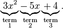
$\underbrace{_\,3x^2}_{\begin{smallmatrix}\mathrm{term}\\\mathrm{1}\end{smallmatrix}} \underbrace{-_\,5x}_{\begin{smallmatrix}\mathrm{term}\\\mathrm{2}\end{smallmatrix}} \underbrace{+_\,4}_{\begin{smallmatrix}\mathrm{term}\\\mathrm{3}\end{smallmatrix}}.$

It consists of three terms: the first is degree two, the second is degree one, and the third is degree zero. Here "− 5x" stands for "+ (−5)x", so the coefficient of the middle term is −5.

When a polynomial in one variable is arranged in the traditional order, the terms of higher degree come before the terms of lower degree. In the first term above, the coefficient is 3, the variable is x, and the exponent is 2. In the second term, the coefficient is –5. The third term is a constant. The degree of a non-zero polynomial is the largest degree of any one term. In this example, the polynomial has degree two.

[edit] Alternative forms

An expression that can be converted to polynomial form through a sequence of applications of the commutative, associative, and distributive laws is usually considered to be a polynomial. For instance,

$(x+1)^3\,$

is a polynomial because it can be worked out to $x 3 + 3 x 2 + 3 x + 1$ . Similarly,

$\frac{x^3}{12}$

is considered a valid term in a polynomial, even though it involves a division, because it is equivalent to $\tfrac{1}{12}x^3$ and $\tfrac{1}{12}$ is just a constant. The coefficient of this term is therefore $\tfrac{1}{12}$ . For similar reasons, if complex coefficients are allowed, one may have a single term like $(2 + 3 i) x 3$ ; even though it looks like it should be worked out to two terms, the complex number 2+3i is in fact just a single coefficient in this case that happens to require a "+" to be written down.

Division by an expression containing a variable is not generally allowed in polynomials.^[1] For example,

${1 \over x^2 + 1} \,$

is not a polynomial because it includes division by a variable. Similarly,

$( 5 + y ) ^ x ,\,$

is not a polynomial, because it has a variable exponent.

Since subtraction can be treated as addition of the additive opposite, and since exponentiation to a constant positive whole number power can be treated as repeated multiplication, polynomials can be constructed from constants and variables with just the two operations addition and multiplication.

[edit] Polynomial functions

A polynomial function is a function defined by evaluating a polynomial. A function ƒ of one argument is called a polynomial function if it satisfies

$f(x) = a_n x^n + a_{n-1} x^{n-1} + \cdots + a_2 x^2 + a_1 x + a_0 \,$

for all arguments x, where n is a nonnegative integer and a₀, a₁,a₂, ..., a_n are constant coefficients.

For example, the function ƒ, taking real numbers to real numbers, defined by

$f(x) = x^3 - x\,$

is a polynomial function of one argument. Polynomial functions of multiple arguments can also be defined, using polynomials in multiple variables, as in

$f(x,y)= 2x^3+4x^2y+xy^5+y^2-7.\,$

Polynomial functions are an important class of smooth functions.

[edit] Polynomial equations

A polynomial equation is an equation in which a polynomial is set equal to another polynomial.

$3x^2 + 4x -5 = 0 \,$

is a polynomial equation. In case of a polynomial equation the variable is considered an unknown, and one seeks to find the possible values for which both members of the equation evaluate to the same value (in general more than one solution may exist). A polynomial equation is to be contrasted with a polynomial identity like (x + y)(x – y) = x²–y², where both members represent the same polynomial in different forms, and as a consequence any evaluation of both members will give a valid equality.

[edit] Elementary properties of polynomials

A sum of polynomials is a polynomial.
A product of polynomials is a polynomial
The derivative of a polynomial function is a polynomial function
Any primitive or antiderivative of a polynomial function is a polynomial function

Polynomials serve to approximate other functions, such as sine, cosine, and exponential.

All polynomials have an expanded form, in which the distributive law has been used to remove all brackets. All polynomials with real or complex coefficients also have a factored form in which the polynomial is written as a product of linear polynomials. For example, the polynomial

$x^2 - 2x - 3 \,$

is the expanded form of the polynomial

$(x - 3)(x + 1)\,$ ,

which is written in factored form. Note that the constants in the linear polynomials (like -3 and +1 in the above example) may be complex numbers in certain cases, even if all coefficients of the expanded form are real numbers. This is because the field of real numbers is not algebraically closed; however, the fundamental theorem of algebra states that the field of complex numbers is algebraically closed.

In school algebra, students learn to move easily from one form to the other (see: factoring).

Every polynomial in one variable is equivalent to a polynomial with the form

$a_n x^n + a_{n-1}x^{n-1} + \cdots + a_2 x^2 + a_1 x + a_0.$

This form is sometimes taken as the definition of a polynomial in one variable.

Evaluation of a polynomial consists of assigning a number to each variable and carrying out the indicated multiplications and additions. Evaluation is sometimes performed more efficiently using the Horner scheme

$((\cdots(a_n x + a_{n-1})x + \cdots + a_2)x + a_1)x + a_0.\,$

In elementary algebra, methods are given for solving all first degree and second degree polynomial equations in one variable. In the case of polynomial equations, the variable is often called an unknown. The number of solutions may not exceed the degree, and will equal the degree when multiplicity of solutions and complex number solutions are counted. This fact is called the fundamental theorem of algebra.

A system of polynomial equations is a set of equations in which a given variable must take on the same value everywhere it appears in any of the equations. Systems of equations are usually grouped with a single open brace on the left. In elementary algebra, methods are given for solving a system of linear equations in several unknowns. To get a unique solution, the number of equations should equal the number of unknowns. If there are more unknowns than equations, the system is called underdetermined. If there are more equations than unknowns, the system is called overdetermined. This important subject is studied extensively in the area of mathematics known as linear algebra. Overdetermined systems are common in practical applications. For example, one U.S. mapping survey used computers to solve 2.5 million equations in 400,000 unknowns.^[2]

[edit] More advanced examples of polynomials

In linear algebra, the characteristic polynomial of a square matrix encodes several important properties of the matrix.

In graph theory the chromatic polynomial of a graph encodes the different ways to vertex color the graph using x colors.

In abstract algebra, one may define polynomials with coefficients in any ring.

In knot theory the Alexander polynomial, the Jones polynomial, and the HOMFLY polynomial are important knot invariants.

[edit] History

Determining the roots of polynomials, or "solving algebraic equations", is among the oldest problems in mathematics. However, the elegant and practical notation we use today only developed beginning in the 15th century. Before that, equations are written out in words. For example, an algebra problem from the Chinese Arithmetic in Nine Sections, circa 200 BCE, begins "Three sheafs of good crop, two sheafs of mediocre crop, and one sheaf of bad crop are sold for 29 dou." We would write $3 x + 2 y + z = 29$ .

[edit] Notation

Main article: History of mathematical notation

The earliest known use of the equal sign is in Robert Recorde's The Whetstone of Witte, 1557. The signs + for addition, − for subtraction, and the use of a letter for an unknown appear in Michael Stifel's Arithemetica integra, 1544. René Descartes, in La géometrie, 1637, introduced the concept of the graph of a polynomial equation. He popularized the use of letters from the beginning of the alphabet to denote constants and letters from the end of the alphabet to denote variables, as can be seen above, in the general formula for a polynomial in one variable, where the a 's denote constants and x denotes a variable. Descartes introduced the use of superscripts to denote exponents as well.^[3]

[edit] Solving polynomial equations

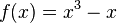
Every polynomial corresponds to a polynomial function, where f(x) is set equal to the polynomial, and to a polynomial equation, where the polynomial is set equal to zero. The solutions to the equation are called the roots of the polynomial and they are the zeroes of the function and the x-intercepts of its graph. If x = a is a root of a polynomial, then (x − a) is a factor of that polynomial.

Some polynomials, such as f(x) = x² + 1, do not have any roots among the real numbers. If, however, the set of allowed candidates is expanded to the complex numbers, every (non-constant) polynomial has at least one distinct root; this follows from the fundamental theorem of algebra.

There is a difference between approximating roots and finding exact roots. Formulas for the roots of polynomials up to a degree of 2 have been known since ancient times (see quadratic equation) and up to a degree of 4 since the 16th century (see Gerolamo Cardano, Niccolo Fontana Tartaglia). But formulas for degree 5 eluded researchers. In 1824, Niels Henrik Abel proved the striking result that there can be no general formula (involving only the arithmetical operations and radicals) for the roots of a polynomial of degree 5 or greater in terms of its coefficients (see Abel-Ruffini theorem). This result marked the start of Galois theory which engages in a detailed study of relationships among roots of polynomials.

Numerically solving a polynomial equation in one unknown is easily done on a computer by the Durand-Kerner method or by some other root-finding algorithm. The reduction of equations in several unknowns to equations each in one unknown is discussed in the article on the Buchberger's algorithm. The special case where all the polynomials are of degree one is called a system of linear equations, for which a range of different solution methods exist, including the classical gaussian elimination.

It has been shown by Richard Birkeland and Karl Meyr that the roots of any polynomial may be expressed in terms of multivariate hypergeometric functions. Ferdinand von Lindemann and Hiroshi Umemura showed that the roots may also be expressed in terms of Siegel modular functions, generalizations of the theta functions that appear in the theory of elliptic functions. These characterizations of the roots of arbitrary polynomials are generalizations of the methods previously discovered to solve the quintic equation.

[edit] Graphs

A polynomial function in one real variable can be represented by a graph.

The graph of the zero polynomial

f(x) = 0

is the x-axis.

The graph of a degree 0 polynomial

f(x) = a₀, where a₀ ≠ 0,

is a horizontal line with y-intercept a₀

The graph of a degree 1 polynomial (or linear function)

f(x) = a₀ + a₁x , where a₁ ≠ 0,

is an oblique line with y-intercept a₀ and slope a₁.

The graph of a degree 2 polynomial

f(x) = a₀ + a₁x + a₂x², where a₂ ≠ 0

is a parabola.

The graph of a degree 3 polynomial

f(x) = a₀ + a₁x + a₂x², + a₃x³, where a₃ ≠ 0

is a cubic curve.

The graph of any polynomial with degree 2 or greater

f(x) = a₀ + a₁x + a₂x² + ... + a_nxⁿ , where a_n ≠ 0 and n ≥ 2

is a continuous non-linear curve.

Polynomial graphs are analyzed in calculus using intercepts, slopes, concavity, and end behavior.

The illustrations below show graphs of polynomials.

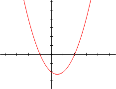
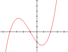
Polynomial of degree 2: f(x) = x² - x - 2 = (x+1)(x-2)	Polynomial of degree 3: f(x) = x³/5 + 4x²/5 - 7x/5 - 2 = 1/5 (x+5)(x+1)(x-2)
Polynomial of degree 4: f(x) = 1/14 (x+4)(x+1)(x-1)(x-3) + 0.5	Polynomial of degree 5: f(x) = 1/20 (x+4)(x+2)(x+1)(x-1)(x-3) + 2

[edit] Polynomials and calculus

Main article: Calculus with polynomials

One important aspect of calculus is the project of analyzing complicated functions by means of approximating them with polynomials. The culmination of these efforts is Taylor's theorem, which roughly states that every differentiable function locally looks like a polynomial, and the Stone-Weierstrass theorem, which states that every continuous function defined on a compact interval of the real axis can be approximated on the whole interval as closely as desired by a polynomial. Polynomials are also frequently used to interpolate functions.

Quotients of polynomials are called rational expressions, and functions that evaluate rational expressions are called rational functions. Rational functions are the only functions that can be evaluated on a computer by a fixed sequence of instructions involving operations of addition, multiplication, division, which operations on floating point numbers are usually implemented in hardware. All the other functions that computers need to evaluate, such as trigonometric functions, logarithms and exponential functions, must then be computed in software that may use approximations to those functions on certain intervals by rational functions, and possibly iteration.

Calculating derivatives and integrals of polynomials is particularly simple. For the polynomial

$\sum_{i=0}^n a_i x^i$

the derivative with respect to x is

$\sum_{i=1}^n a_i i x^{i-1}$

and the indefinite integral is

$\sum_{i=0}^n {a_i\over i+1} x^{i+1}+c.$

[edit] Abstract algebra

Main article: Polynomial ring

In abstract algebra, one must take care to distinguish between polynomials and polynomial functions. A polynomial f in one variable $X$ over a ring $R$ is defined to be a formal expression of the form

$f = a_n X^n + a_{n - 1} X^{n - 1} + \cdots + a_1 X^1 + a_0X^0$

where $n$ is a natural number, the coefficients $a_0,\ldots,a_n$ are elements of $R$ , Here X is a formal symbol, whose powers Xⁱ are at this point just placeholders for the corresponding coefficients a_i, so that the given formal expression is just a way to encode the sequence (a₀,a₁,...), where there is an N such that a_i=0 for all i>N. Two polynomials sharing the same value of $n$ are considered to be equal if and only if the sequences of their coefficients are equal; furthermore any polynomial is equal to any polynomial with greater value of $n$ obtained from it by adding terms in front whose coefficient is zero. These polynomials can be added by simply adding corresponding coefficients (the rule for extending by terms with zero coefficients can be used to make sure such coefficients exist). Thus each polynomial is actually equal to the sum of the terms used in its formal expression, if such a term a_iXⁱ is interpreted as a polynomial that has zero coefficients at all powers of X other than Xⁱ. Then to define multiplication, it suffices by the distributive law to describe the product of any two such terms, which is given by the rule

$a X^k \; b X^l = ab X^{k+l}$

for all elements a, b of the ring R and all natural numbers k and l.

Thus the set of all polynomials with coefficients in the ring R forms itself a ring, the ring of polynomials over R, which is denoted by R[X]. The map from R to R[X] sending r to rX⁰ is an injective homomorphism of rings, by which R is viewed as a subring of R[X]. If R is commutative, then R[X] is an algebra over R.

One can think of the ring R[X] as arising from R by adding one new element X to R, and extending in a minimal way to a ring in which X satisfies no other relations than the obligatory ones, plus commutation with all elements of R (that is Xr = rX). To do this, one must add all powers of X and their linear combinations as well.

Formation of the polynomial ring, together with forming factor rings by factoring out ideals, are important tools for constructing new rings out of known ones. For instance, the ring (in fact field) of complex numbers, which can be constructed from the polynomial ring R[X] over the real numbers by factoring out the ideal of multiples of the polynomial X² + 1. Another example is the construction of finite fields, which proceeds similarly, starting out with the field of integers modulo some prime number as the coefficient ring R (see modular arithmetic).

If $R$ is commutative, then one can associate to every polynomial P in $R [X]$ , a polynomial function f with domain and range equal to $R$ (more generally one can take domain and range to be the same unital associative algebra over $R$ ). One obtains the value f(r) by everywhere replacing the symbol X in P by r. One reason that algebraists distinguish between polynomials and polynomial functions is that over some rings different polynomials may give rise to the same polynomial function (see Fermat's little theorem for an example where R is the integers modulo p). This is not the case when $R$ is the real or complex numbers and therefore many analysts often don't separate the two concepts. An even more important reason to distinguish between polynomials and polynomial functions is that many operations on polynomials (like Euclidean division) require looking at what a polynomial is composed of as an expression rather than evaluating it at some constant value for $X$ . And it should be noted that if $R$ is not commutative, there is no (well behaved) notion of polynomial function at all.

[edit] Divisibility

In commutative algebra, one major focus of study is divisibility among polynomials. If R is an integral domain and f and g are polynomials in R[X], it is said that f divides g if there exists a polynomial q in R[X] such that f q = g. One can then show that "every zero gives rise to a linear factor", or more formally: if f is a polynomial in R[X] and r is an element of R such that f(r) = 0, then the polynomial (X − r) divides f. The converse is also true. The quotient can be computed using the Horner scheme.

If F is a field and f and g are polynomials in F[X] with g ≠ 0, then there exist unique polynomials q and r in F[X] with

$f = q \, g + r$

and such that the degree of r is smaller than the degree of g. The polynomials q and r are uniquely determined by f and g. This is called "division with remainder" or "polynomial long division" and shows that the ring F[X] is a Euclidean domain.

Analogously, polynomial "primes" (more correctly, irreducible polynomials) can be defined which cannot be factorized into the product of two polynomials of lesser degree. It is not easy to determine if a given polynomial is irreducible. One can start by simply checking if the polynomial has linear factors. Then, one can check divisibility by some other irreducible polynomials. Eisenstein's criterion can also be used in some cases to determine irreducibility.

[edit] Classifications

The most important classification of polynomials is based on the number of distinct variables. A polynomial in one variable is called a univariate polynomial, a polynomial in more than one variable is called a multivariate polynomial. These notions refer more to the kind of polynomials one is generally working with than to individual polynomials; for instance when working with univariate polynomials one does not exclude constant polynomials (which may result for instance from the subtraction of non-constant polynomials), although strictly speaking constant polynomials do not contain any variables at all. It is possible to further classify multivariate polynomials as bivariate, trivariate etc., according to the number of variables, but this is rarely done; it is more common for instance to say simply "polynomials in x, y, and z". A (usually multivariate) polynomial is called homogeneous of degree n if all its terms have degree n.

Univariate polynomials have many properties not shared by multivariate polynomials. For instance, the terms of a univariate polynomial are completely ordered by their degree, and it is conventional to always write them in order of decreasing degree. A univariate polynomial in x of degree n then takes the general form

$c_nx^n+c_{n-1}x^{n-1}+\cdots+c_2x^2+c_1x+c_0$

where c_n, c_n-1, ..., c₂, c₁ and c₀ are constants, the coefficients of this polynomial. Here the term c_nxⁿ is called the leading term and its coefficient c_n the leading coefficient; if the leading coefficient is 1, the univariate polynomial is called monic. Note that apart from the leading coefficient c_n (which must be non-zero or else the polynomial would not be of degree n) this general form allows for coefficients to be zero; when this happens the corresponding term is zero and may be removed from the sum without changing the polynomial. It is nevertheless common to refer to c_i as the coefficient of xⁱ, even when c_i happens to be 0, so that xⁱ does not really occur in any term; for instance one can speak of the constant term of the polynomial, meaning c₀ even if it should be zero.

Polynomials can similarly be classified by the kind of constant values allowed as coefficients. One can work with polynomials with integral, rational, real or complex coefficients, and in abstract algebra polynomials with many other types of coefficients can be defined. Like for the previous classification, this is about the coefficients one is generally working with; for instance when working with polynomials with complex coefficients one includes polynomials whose coefficients happen to all be real, even though such polynomials can also be considered to be a polynomials with real coefficients.

Polynomials can further be classified by their degree and/or the number of non-zero terms they contain.

Polynomials classified by degree
Degree	Name	Example
−∞	zero	$0$
$0$	(non-zero) constant	$1$
$1$	linear	$x + 1$
$2$	quadratic	$x 2 + 1$
$3$	cubic	$x 3 + 1$
$4$	quartic (or biquadratic)	$x 4 + 1$
$5$	quintic	$x 5 + 1$
$6$	sextic or hexic	$x 6 + 1$
$7$	septic or heptic	$x 7 + 1$
$8$	octic	$x 8 + 1$
$9$	nonic	$x 9 + 1$
$10$	decic	$x 10 + 1$

Usually, a polynomial of degree 4 or higher is referred to as a polynomial of degree n, although the phrases quartic polynomial and quintic polynomial are also used. The names for degrees higher than 5 are even less common. The names for the degrees may be applied to the polynomial or to its terms. For example, a constant may refer to a zero degree polynomial or to a zero degree term.

The polynomial 0, which may be considered to have no terms at all, is called the zero polynomial. Unlike other constant polynomials, its degree is not zero. Rather the degree of the zero polynomial is either left explicitly undefined, or defined to be negative (either –1 or –∞).^[4] The latter convention is important when defining Euclidean division of polynomials.

Polynomials classified by number of non-zero terms
Number of non-zero terms	Name	Example
$0$	zero polynomial	$0$
$1$	monomial	$x 2$
$2$	binomial	$x 2 + 1$
$3$	trinomial	$x 2 + x + 1$

The word monomial can be ambiguous, as it is also often used to denote just a power of the variable, or in the multivariate case product of such powers, without any coefficient. Two or more terms which involve the same monomial in the latter sense, in other words which differ only in the value of their coefficients, are called similar terms; they can be combined into a single term by adding their coefficients; if the resulting term has coefficient zero, it may be removed altogether. The above classification according to the number of terms assumes that similar terms have been combined first.

[edit] Polynomials associated to other objects

Polynomials are frequently used to encode information about some other object. The characteristic polynomial of a matrix or linear operator contains information about the operator's eigenvalues. The minimal polynomial of an algebraic element records the simplest algebraic relation satisfied by that element. The chromatic polynomial of a graph counts the number of proper colourings of that graph.

[edit] Extensions of the concept of a polynomial

Polynomials can involve more than one variable, in which they are called multivariate. Rings of polynomials in a finite number of variables are of fundamental importance in algebraic geometry which studies the simultaneous zero sets of several such multivariate polynomials. These rings can alternatively be constructed by repeating the construction of univariate polynomials with as ceofficient ring another ring of polynomials: thus the ring R[X,Y] of polynomials in X and Y can be viewed as the ring (R[X])[Y] of polynomials in Y with as coeffcients polynomials in X, or as the ring (R[Y])[X] of polynomials in X with as coeffcients polynomials in Y. These identifications are compatible with arithmetic operations (they are isomorphisms of rings), but some notions such as degree or whether a polynomial is considered monic can change between these points of view. One can construct rings of polynomials in infinitely many variables, but since polynomials are (finite) expressions, any individual polynomial can only contain finitely many variables.

Laurent polynomials are like polynomials, but allow negative powers of the variable(s) to occur.

Rational functions are formal quotients of polynomials (they are formed from polynomials just as rational numbers are formed from integers, writing a fraction of two of them; fractions related by the cancelling of common factors are identified with each other). The rational functions contain the Laurent polynomials, but do not limit denominators to be powers of a variable.

Formal power series are like polynomials, but allow infinitely many nonzero terms to occur, so that they do not have finite degree. Unlike polynomials they cannot in general be explicitly and fully written down (just like real numbers cannot), but the rules for manipulating their terms are the same as for polynomials.

[edit] See also

Please see List of polynomial topics

[edit] Notes

^ Peter H. Selby, Steve Slavin, Practical Algebra: A Self-Teaching Guide, 2nd Edition, Wiley, ISBN-10 0471530123 ISBN-13 978-0471530121
^ Gilbert Strang, Linear Algebra and its Applications, Fourth Edition, Thompson Brooks/Cole, ISBN 0030105676.
^ Howard Eves, An Introduction to the History of Mathematics, Sixth Edition, Saunders, ISBN 0030295580
^ http://mathworld.wolfram.com/ZeroPolynomial.html

[edit] References

R. Birkeland. Über die Auflösung algebraischer Gleichungen durch hypergeometrische Funktionen. Mathematische Zeitschrift vol. 26, (1927) pp. 565-578. Shows that the roots of any polynomial may be written in terms of multivariate hypergeometric functions. Paper is available here.
F. von Lindemann. Über die Auflösung der algebraischen Gleichungen durch transcendente Functionen. Nachrichten von der Königl. Gesellschaft der Wissenschaften, vol. 7, 1884. Polynomial solutions in terms of theta functions. Paper available here.
F. von Lindemann. Über die Auflösung der algebraischen Gleichungen durch transcendente Functionen II. Nachrichten von der Königl. Gesellschaft der Wissenschaften und der Georg-Augusts-Universität zu Göttingen, 1892 edition. Paper available here.
K. Mayr. Über die Auflösung algebraischer Gleichungssysteme durch hypergeometrische Funktionen. Monatshefte für Mathematik und Physik vol. 45, (1937) pp. 280-313.
H. Umemura. Solution of algebraic equations in terms of theta constants. In D. Mumford, Tata Lectures on Theta II, Progress in Mathematics 43, Birkhäuser, Boston, 1984.

[edit] External links

[0] Peter H. Selby, Steve Slavin, Practical Algebra: A Self-Teaching Guide, 2nd Edition, Wiley, ISBN-10 0471530123 ISBN-13 978-0471530121

[1] Gilbert Strang, Linear Algebra and its Applications, Fourth Edition, Thompson Brooks/Cole, ISBN 0030105676.

[2] Howard Eves, An Introduction to the History of Mathematics, Sixth Edition, Saunders, ISBN 0030295580

[3] ttp://mathworld.wolfram.com/ZeroPolynomial.html

[1]

[2]

[3]

[4]