Global Positioning System

From Wikipedia, the free encyclopedia

"GPS" redirects here. For other similar systems, see Global Navigation Satellite System. For other uses of "GPS", see GPS (disambiguation).

For a generally accessible and less technical introduction to the topic, see Introduction to the Global Positioning System.

Artist's conception of GPS Block II-F satellite in orbit

Civilian GPS receiver ("GPS navigation device") in a marine application.

Automotive navigation system in a taxicab.

GPS receivers are now integrated in many mobile phones.

The Global Positioning System (GPS) is a global navigation satellite system (GNSS) developed by the United States Department of Defense and managed by the United States Air Force 50th Space Wing. It is the only fully functional GNSS in the world, can be used freely, and is often used by civilians for navigation purposes. It uses a constellation of between 24 and 32 Medium Earth Orbit satellites that transmit precise radiowave signals, which allow GPS receivers to determine their current location, the time, and their velocity. Its official name is NAVSTAR GPS. Although NAVSTAR is not an acronym,^[1] a few backronyms have been created for it.^[2]

Since it became fully operational in 1993, GPS has become a widely used aid to navigation worldwide, and a useful tool for map-making, land surveying, commerce, scientific uses, and hobbies such as geocaching. Also, the precise time reference is used in many applications including the scientific study of earthquakes. GPS is also a required key synchronization resource of cellular networks, such as the Qualcomm CDMA air interface used by many wireless carriers in a multitude of countries.^{[citation needed]}

1 History
- 1.1 Timeline
2 Basic concept of GPS
- 2.1 Position calculation introduction
- 2.2 Correcting a GPS receiver's clock
3 System detail
4 Possible Sources of Interference
- 4.1 Natural sources
- 4.2 Artificial sources
5 Accuracy enhancement
6 Applications
- 6.1 Military
- 6.2 Civilian
7 Awards
8 Other systems
9 Multidimensional Newton-Raphson for GPS
10 See also
11 References
12 External links

[edit] History

The first satellite navigation system, Transit, used by the United States Navy, was first successfully tested in 1960. Using a constellation of five satellites, it could provide a navigational fix approximately once per hour. In 1967, the U.S. Navy developed the Timation satellite which proved the ability to place accurate clocks in space, a technology that GPS relies upon. In the 1970s, the ground-based Omega Navigation System, based on signal phase comparison, became the first worldwide radio navigation system.

The design of GPS is based partly on similar ground-based radio navigation systems, such as LORAN and the Decca Navigator developed in the early 1940s, and used during World War II. Additional inspiration for the GPS came when the Soviet Union launched the first Sputnik in 1957. A team of U.S. scientists led by Dr. Richard B. Kershner were monitoring Sputnik's radio transmissions. They discovered that, because of the Doppler effect, the frequency of the signal being transmitted by Sputnik was higher as the satellite approached, and lower as it continued away from them. They realized that since they knew their exact location on the globe, they could pinpoint where the satellite was along its orbit by measuring the Doppler distortion.

After Korean Air Lines Flight 007 was shot down in 1983 after straying into the USSR's prohibited airspace,^[3] President Ronald Reagan issued a directive making GPS freely available for civilian use as a common good.^[4] The satellites were launched between 1989 and 1993.

Initially the highest quality signal was reserved for military use, while the signal available for civilian use was intentionally degraded ("Selective Availability", SA). Selective Availability was ended in 2000, improving the precision of civilan GPS from about 100m to about 20m.

Of crucial importance for the function of GPS is the placement of atomic clocks in the satellites, first proposed by Friedwardt Winterberg in 1955.^[5] Only then can the required position accuracy be reached.

[edit] Timeline

In 1972, the US Air Force Central Inertial Guidance Test Facility (Holloman AFB) conducted developmental flight tests of two prototype GPS receivers over White Sands Missile Range, using ground-based pseudo-satellites.

Satellite numbers^[6]^[7]^[8]
Block	Launch Period	Satellites launched	Currently in service
I	1978–1985	10+1¹	0
II	1985–1990	9	0
IIA	1990–1997	19	13
IIR	1997–2004	12+1¹	12
IIR-M	2005–2009	7+1²	6
IIF	2009–2011	0+10²	0
IIIA	2014–?	0+12³	0
IIIB		0+8³	0
IIIC		0+16³	0
Total		59+2¹+12²+36³	31
¹Failed ²In preparation ³Planned. (Last update: 16 December 2008)

In 1978 the first experimental Block-I GPS satellite was launched.
In 1983, after Soviet interceptor aircraft shot down the civilian airliner KAL 007 that strayed into prohibited airspace due to navigational errors, killing all 269 people on board, U.S. President Ronald Reagan announced that the GPS would be made available for civilian uses once it was completed.^[9]^[10]
By 1985, ten more experimental Block-I satellites had been launched to validate the concept.
On February 14, 1989, the first modern Block-II satellite was launched.
In 1992, the 2nd Space Wing, which originally managed the system, was de-activated and replaced by the 50th Space Wing.
By December 1993 the GPS achieved initial operational capability.^[11]
By January 17, 1994 a complete constellation of 24 satellites was in orbit.
Full Operational Capability was declared by NAVSTAR in April 1995.
In 1996, recognizing the importance of GPS to civilian users as well as military users, U.S. President Bill Clinton issued a policy directive^[12] declaring GPS to be a dual-use system and establishing an Interagency GPS Executive Board to manage it as a national asset.
In 1998, U.S. Vice President Al Gore announced plans to upgrade GPS with two new civilian signals for enhanced user accuracy and reliability, particularly with respect to aviation safety.
On May 2, 2000 "Selective Availability" was discontinued as a result of the 1996 executive order, allowing users to receive a non-degraded signal globally.
In 2004, the United States Government signed an agreement with the European Community establishing cooperation related to GPS and Europe's planned Galileo system.
In 2004, U.S. President George W. Bush updated the national policy and replaced the executive board with the National Space-Based Positioning, Navigation, and Timing Executive Committee.
November 2004, QUALCOMM announced successful tests of Assisted-GPS for mobile phones.^[13]
In 2005, the first modernized GPS satellite was launched and began transmitting a second civilian signal (L2C) for enhanced user performance.
On September 14, 2007, the aging mainframe-based Ground Segment Control System was transitioned to the new Architecture Evolution Plan.^[14]
The most recent launch was on March 15, 2008.^[15] The oldest GPS satellite still in operation was launched on November 26, 1990, and became operational on December 10, 1990.^[16]

[edit] Basic concept of GPS

A GPS receiver calculates its position by precisely timing the signals sent by the GPS satellites high above the Earth. Each satellite continually transmits messages containing the time the message was sent, precise orbital information (the ephemeris), and the general system health and rough orbits of all GPS satellites (the almanac). The receiver measures the transit time of each message and computes the distance to each satellite. Geometric trilateration is used to combine these distances with the location of the satellites to determine the receiver's location. The position is displayed, perhaps with a moving map display or latitude and longitude; elevation information may be included. Many GPS units also show derived information such as direction and speed, calculated from position changes.

It might seem three satellites are enough to solve for position, since space has three dimensions. However a very small clock error multiplied by the very large speed of light^[17]—the speed at which satellite signals propagate—results in a large positional error. The receiver uses a fourth satellite to solve for x, y, z, and t which is used to correct the receiver's clock. While most GPS applications use the computed location only and effectively hide the very accurately computed time, it is used in a few specialized GPS applications such as time transfer and traffic signal timing.

Although four satellites are required for normal operation, fewer apply in special cases. If one variable is already known (for example, a ship or plane may have known elevation), a receiver can determine its position using only three satellites. Some GPS receivers may use additional clues or assumptions (such as reusing the last known altitude, dead reckoning, inertial navigation, or including information from the vehicle computer) to give a degraded position when fewer than four satellites are visible (see ^[18], Chapters 7 and 8 of ^[19], and ^[20]).

[edit] Position calculation introduction

To provide an introductory description of how a GPS receiver works, measurement errors will be ignored in this section. Using messages received from a minimum of four visible satellites, a GPS receiver is able to determine the satellite positions and time sent. The x, y, and z components of position and the time sent are designated as $\left [x_i, y_i, z_i, t_i\right ]$ where the subscript i is the satellite number and has the value 1, 2, 3, or 4. Knowing the indicated time the message was received $\ tr_i$ , the GPS receiver can compute the indicated transit time, $\left (tr_i-t_i\right )$ . of the message. Assuming the message traveled at the speed of light, c, the distance traveled, $\ p_i$ can be computed as $\left (tr_i-t_i\right )c$ . 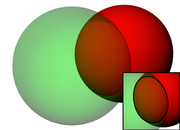Knowing the distance from GPS receiver to a satellite and the position of a satellite implies that the GPS receiver is on the surface of a sphere centered at the position of a satellite. Thus we know that the indicated position of the GPS receiver is at or near the intersection of the surfaces of four spheres. In the ideal case of no errors, the GPS receiver will be at an intersection of the surfaces of four spheres. The surfaces of two spheres, if they intersect in more than one point, intersect in a circle. A figure, Two Sphere Surfaces Intersecting in a Circle, is shown below.

Two sphere surfaces intersecting in a circle

The article, trilateration, shows mathematically that the surfaces of two spheres, intersecting in more than one point, intersect in a circle.

Surface of a sphere intersecting a circle (i.e., the edge of a disk) at two points

A circle and sphere surface in most cases of practical interest intersect at two points, although it is conceivable that they could intersect at one point—or not at all, or at the entire circle. Another figure, Surface of Sphere Intersecting a Circle (not disk) at Two Points, shows this intersection. The two intersections are marked with dots. Again trilateration clearly shows this mathematically. The correct position of the GPS receiver is the intersection that is closest to the surface of the earth for automobiles and other near-Earth vehicles. The correct position of the GPS receiver is also the intersection which is closest to the surface of the sphere corresponding to the fourth satellite. (The two intersections are symmetrical with respect to the plane containing the three satellites. If the three satellites are not in the same orbital plane, the plane containing the three satellites will not be a vertical plane passing through the center of the Earth. In this case one of the intersections will be closer to the earth than the other. The near-Earth intersection will be the correct position for the case of a near-Earth vehicle. The intersection which is farthest from Earth may be the correct position for space vehicles.)

[edit] Correcting a GPS receiver's clock

The method of calculating position for the case of no errors has been explained. One of the most significant error sources is the GPS receiver's clock. Because of the very large value of the speed of light, c, the estimated distances from the GPS receiver to the satellites, the pseudoranges, are very sensitive to errors in the GPS receiver clock. This suggests that an extremely accurate and expensive clock is required for the GPS receiver to work. On the other hand, manufacturers prefer to build inexpensive GPS receivers for mass markets. The solution for this dilemma is based on the way sphere surfaces intersect in the GPS problem.

It is likely the surfaces of the three spheres intersect since the circle of intersection of the first two spheres is normally quite large and thus the third sphere surface is likely to intersect this large circle. It is very unlikely that the surface of the sphere corresponding to the fourth satellite will intersect either of the two points of intersection of the first three since any clock error could cause it to miss intersecting a point. However the distance from the valid estimate of GPS receiver position to the surface of the sphere corresponding to the fourth satellite can be used to compute a clock correction. Let $\ r_4$ denote the distance from the valid estimate of GPS receiver position to the fourth satellite and let $\ p_4\$ denote the pseudorange of the fourth satellite. Let $\ da = r_4 - p_4$ . Note that $\ da$ is the distance from the computed GPS receiver position to the surface of the sphere corresponding to the fourth satellite. Thus the quotient, $\ b = da / c\$ , provides an estimate of

(correct time) - (time indicated by the receiver's on-board clock), and the GPS receiver clock can be advanced if $\ b$ is positive or delayed if $\ b$ is negative.

[edit] System detail

Unlaunched GPS satellite on display at the San Diego Aerospace museum

[edit] System segmentation

The current GPS consists of three major segments. These are the space segment (SS), a control segment (CS), and a user segment (US).^[21]

[edit] Space segment

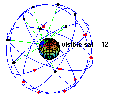
A visual example of the GPS constellation in motion with the Earth rotating. Notice how the number of satellites in view from a given point on the Earth's surface, in this example at 45°N, changes with time.

The space segment (SS) comprises the orbiting GPS satellites, or Space Vehicles (SV) in GPS parlance. The GPS design originally called for 24 SVs, eight each in three circular orbital planes,^[22] but this was modified to six planes with four satellites each.^[23] The orbital planes are centered on the Earth, not rotating with respect to the distant stars.^[24] The six planes have approximately 55° inclination (tilt relative to Earth's equator) and are separated by 60° right ascension of the ascending node (angle along the equator from a reference point to the orbit's intersection).^[25] The orbits are arranged so that at least six satellites are always within line of sight from almost everywhere on Earth's surface.^[26]

Orbiting at an altitude of approximately 20,200 kilometers about 10 satellites are visible within line of sight (12,600 miles or 10,900 nautical miles; orbital radius of 26,600 km (16,500 mi or 14,400 NM)), each SV makes two complete orbits each sidereal day.^[27] The ground track of each satellite therefore repeats each (sidereal) day. This was very helpful during development, since even with just four satellites, correct alignment means all four are visible from one spot for a few hours each day. For military operations, the ground track repeat can be used to ensure good coverage in combat zones.

As of March 2008^[update],^[28] there are 31 actively broadcasting satellites in the GPS constellation, and two older, retired from active service satellites kept in the constellation as orbital spares. The additional satellites improve the precision of GPS receiver calculations by providing redundant measurements. With the increased number of satellites, the constellation was changed to a nonuniform arrangement. Such an arrangement was shown to improve reliability and availability of the system, relative to a uniform system, when multiple satellites fail.^[29]

[edit] Control segment

The flight paths of the satellites are tracked by US Air Force monitoring stations in Hawaii, Kwajalein, Ascension Island, Diego Garcia, and Colorado Springs, Colorado, along with monitor stations operated by the National Geospatial-Intelligence Agency (NGA).^[30] The tracking information is sent to the Air Force Space Command's master control station at Schriever Air Force Base in Colorado Springs, which is operated by the 2nd Space Operations Squadron (2 SOPS) of the United States Air Force (USAF). Then 2 SOPS contacts each GPS satellite regularly with a navigational update (using the ground antennas at Ascension Island, Diego Garcia, Kwajalein, and Colorado Springs). These updates synchronize the atomic clocks on board the satellites to within a few nanoseconds of each other, and adjust the ephemeris of each satellite's internal orbital model. The updates are created by a Kalman filter which uses inputs from the ground monitoring stations, space weather information, and various other inputs.^[31]

Satellite maneuvers are not precise by GPS standards. So to change the orbit of a satellite, the satellite must be marked 'unhealthy', so receivers will not use it in their calculation. Then the maneuver can be carried out, and the resulting orbit tracked from the ground. Then the new ephemeris is uploaded and the satellite marked healthy again.

[edit] User segment

GPS receivers come in a variety of formats, from devices integrated into cars, phones, and watches, to dedicated devices such as those shown here from manufacturers Trimble, Garmin and Leica (left to right).

The user's GPS receiver is the user segment (US) of the GPS. In general, GPS receivers are composed of an antenna, tuned to the frequencies transmitted by the satellites, receiver-processors, and a highly-stable clock (often a crystal oscillator). They may also include a display for providing location and speed information to the user. A receiver is often described by its number of channels: this signifies how many satellites it can monitor simultaneously. Originally limited to four or five, this has progressively increased over the years so that, as of 2007^[update], receivers typically have between 12 and 20 channels.^[32]

A typical OEM GPS receiver module measuring 15×17 mm.

GPS receivers may include an input for differential corrections, using the RTCM SC-104 format. This is typically in the form of a RS-232 port at 4,800 bit/s speed. Data is actually sent at a much lower rate, which limits the accuracy of the signal sent using RTCM. Receivers with internal DGPS receivers can outperform those using external RTCM data. As of 2006, even low-cost units commonly include Wide Area Augmentation System (WAAS) receivers.

A typical GPS receiver with integrated antenna.

Many GPS receivers can relay position data to a PC or other device using the NMEA 0183 protocol, or the newer and less widely used NMEA 2000.^[33] Although these protocols are officially defined by the NMEA,^[34] references to these protocols have been compiled from public records, allowing open source tools like gpsd to read the protocol without violating intellectual property laws. Other proprietary protocols exist as well, such as the SiRF and MTK protocols. Receivers can interface with other devices using methods including a serial connection, USB or Bluetooth.

[edit] Navigation signals

GPS broadcast signal

Each GPS satellite continuously broadcasts a Navigation Message at 50 bit/s giving the time-of-week, GPS week number and satellite health information (all transmitted in the first part of the message), an ephemeris (transmitted in the second part of the message) and an almanac (later part of the message). The messages are sent in frames, each taking 30 seconds to transmit 1500 bits.

Transmission of each 30 second frame begins precisely on the minute and half minute as indicated by the satellite's atomic clock according to Satellite message format. Each frame contains 5 subframes of length 6 seconds and with 300 bits. Each subframe contains 10 words of 30 bits with length 0.6 seconds each.

Words 1 and 2 of every subframe have the same type of data. The first word is the telemetry word which indicates the beginning of a subframe and is used by the receiver to synch with the navigation message. The second word is the HOW or handover word and it contains timing information which enables the receiver to identify the subframe and provides the time the next subframe was sent.

Words 3 through 10 of subframe 1 contain data describing the satellite clock and its relationship to GPS time. Words 3 through 10 of subframes 2 and 3, contain the ephemeris data, giving the satellite's own precise orbit. The ephemeris is updated every 2 hours and is generally valid for 4 hours, with provisions for updates every 6 hours or longer in non-nominal conditions. The time needed to acquire the ephemeris is becoming a significant element of the delay to first position fix, because, as the hardware becomes more capable, the time to lock onto the satellite signals shrinks, but the ephemeris data requires 30 seconds (worst case) before it is received, due to the low data transmission rate.

The almanac consists of coarse orbit and status information for each satellite in the constellation, an ionospheric model, and information to relate GPS derived time to Coordinated Universal Time (UTC). Words 3 through 10 of subframes 4 and 5 contain a new part of the almanac. Each frame contains 1/25th of the almanac, so 12.5 minutes are required to receive the entire almanac from a single satellite.^[35] The almanac serves several purposes. The first is to assist in the acquisition of satellites at power-up by allowing the receiver to generate a list of visible satellites based on stored position and time, while an ephemeris from each satellite is needed to compute position fixes using that satellite. In older hardware, lack of an almanac in a new receiver would cause long delays before providing a valid position, because the search for each satellite was a slow process. Advances in hardware have made the acquisition process much faster, so not having an almanac is no longer an issue. The second purpose is for relating time derived from the GPS (called GPS time) to the international time standard of UTC. Finally, the almanac allows a single-frequency receiver to correct for ionospheric error by using a global ionospheric model. The corrections are not as accurate as augmentation systems like WAAS or dual-frequency receivers. However, it is often better than no correction, since ionospheric error is the largest error source for a single-frequency GPS receiver. An important thing to note about navigation data is that each satellite transmits not only its own ephemeris, but transmits an almanac for all satellites.

All satellites broadcast at the same two frequencies, 1.57542 GHz (L1 signal) and 1.2276 GHz (L2 signal). The receiver can distinguish the signals from different satellites because GPS uses a code division multiple access (CDMA) spread-spectrum technique where the low-bitrate message data is encoded with a high-rate pseudo-random (PRN) sequence that is different for each satellite. The receiver knows the PRN codes for each satellite and can use this to reconstruct the actual message data. The message data is transmitted at 50 bits per second. Two distinct CDMA encodings are used: the coarse/acquisition (C/A) code (a so-called Gold code) at 1.023 million chips per second, and the precise (P) code at 10.23 million chips per second. The L1 carrier is modulated by both the C/A and P codes, while the L2 carrier is only modulated by the P code.^[36] The C/A code is public and used by civilian GPS receivers, while the P code can be encrypted as a so-called P(Y) code which is only available to military equipment with a proper decryption key. Both the C/A and P(Y) codes impart the precise time-of-day to the user.

[edit] Satellite frequencies

L1 (1575.42 MHz): Mix of Navigation Message, coarse-acquisition (C/A) code and encrypted precision P(Y) code, plus the new L1C on future Block III satellites.
L2 (1227.60 MHz): P(Y) code, plus the new L2C code on the Block IIR-M and newer satellites.
L3 (1381.05 MHz): Used by the Nuclear Detonation (NUDET) Detection System Payload (NDS) to signal detection of nuclear detonations and other high-energy infrared events. Used to enforce nuclear test ban treaties.
L4 (1379.913 MHz): Being studied for additional ionospheric correction.
L5 (1176.45 MHz): Proposed for use as a civilian safety-of-life (SoL) signal (see GPS modernization). This frequency falls into an internationally protected range for aeronautical navigation, promising little or no interference under all circumstances. The first Block IIF satellite that would provide this signal is set to be launched in 2009.^[37]

[edit] C/A code

[edit] Demodulation and decoding

Demodulating and Decoding GPS Satellite Signals using the Coarse/Acquisition Gold code.

Since all of the satellite signals are modulated onto the same L1 carrier frequency, there is a need to separate the signals after demodulation. This is done by assigning each satellite a unique pseudorandom sequence known as a Gold code, and the signals are decoded, after demodulation, using modulo 2 addition of the Gold codes corresponding to satellites n₁ through n_k, where k is the number of channels in the GPS receiver and n₁ through n_k are the pseudorandom numbers associated with the satellites. The results of these modulo 2 additions are the 50 bit/s navigation messages from satellites n₁ through n_k. The Gold codes used in GPS are a sequence of 1023 bits with a period of one millisecond. These Gold codes are highly mutually orthogonal, so that it is unlikely that one satellite signal will be misinterpreted as another. As well, the Gold codes have good auto-correlation properties.^[38]

There are 1025 different Gold codes of length 1023 bits, but only 32 are used. These Gold codes are quite often referred to as pseudo random noise since they contain no data and are said to look like random sequences^[39]. However, this may be misleading since they are actually deterministic sequences.

If the almanac information has previously been acquired, the receiver picks which satellites to listen for by their PRN numbers. If the almanac information is not in memory, the receiver enters a search mode and cycles through the PRN numbers until a lock is obtained on one of the satellites. To obtain a lock, it is necessary that there be an unobstructed line of sight from the receiver to the satellite. The receiver can then acquire the almanac and determine the satellites it should listen for. As it detects each satellite's signal, it identifies it by its distinct C/A code pattern.

The receiver uses the C/A Gold code with the same PRN number as the satellite to compute an offset, O, that generates the best correlation. The offset, O, is computed in a trial and error manner. The 1023 bits of the satellite PRN signal are compared with the receiver PRN signal. If correlation is not achieved, the 1023 bits of the receiver's internally generated PRN code are shifted by one bit relative to the satellite's PRN code and the signals are again compared. This process is repeated until correlation is achieved or all 1023 possible cases have been tried (see "How a GPS Receiver Gets a Lock"). If all 1023 cases have been tried without achieving correlation, the frequency oscillator is offset to the next value and the process is repeated.

Since the carrier frequency received can vary due to Doppler shift, the points where received PRN sequences begin may not differ from O by an exact integral number of milliseconds. Because of this, carrier frequency tracking along with PRN code tracking are used to determine when the received satellite's PRN code begins (see "How a GPS Receiver Gets a Lock"). Unlike the earlier computation of offset in which trials of all 1023 offsets could potentially be required, the tracking to maintain lock usually requires shifting of half a pulse width or less. To perform this tracking, the receiver observes two quantities, phase error and received frequency offset. The correlation of the received PRN code with respect to the receiver generated PRN code is computed to determine if the bits of the two signals are misaligned. Comparisons with correlation computed with receiver generated PRN code shifted half a pulse width early and half a pulse width late (see section 1.4.2.4 of ^[19]) are used to estimate adjustment required. The amount of adjustment required for maximum correlation is used in estimating phase error. Received frequency offset from the frequency generated by the receiver provides an estimate of phase rate error. The command for the frequency generator and any further PRN code shifting required are computed as a function of the phase error and the phase rate error in accordance with the control law used. The Doppler velocity is computed as a function of the frequency offset from the carrier nominal frequency. The Doppler velocity is the velocity component along the line of sight of the receiver relative to the satellite.

As the receiver continues to read successive PRN sequences, it will encounter a sudden change in the phase of the 1023 bit received PRN signal. This indicates the beginning of a data bit of the navigation message (see section 1.4.2.5 of ^[19]). This enables the receiver to begin reading the 20 millisecond bits of the navigation message. Each subframe of the navigation frame begins with a Telemetry Word which enables the receiver to detect the beginning of a subframe and determine the receiver clock time at which the navigation subframe begins. Also each subframe of the navigation frame is identified by bits in the Handover Word (HOW) thereby enabling the receiver to determine which subframe (see section 1.4.2.6 of ^[19] and section 2.5.4 of "Essentials of Satellite Navigation Compendium"). There can be a delay of up to 30 seconds before the first estimate of position because of the need to read the ephemeris data before computing the intersections of sphere surfaces.

After a subframe has been read and interpreted, the time the next subframe was sent can be calculated through the use of the clock correction data and the HOW word. The receiver knows the receiver clock time of when the beginning of the next subframe was received from detection of the Telemetry Word thereby enabling computation of the transit time and thus the pseudorange. The receiver is potentially capable of getting a new pseudorange measurement at the beginning of each subframe or every 6 seconds.

Then the orbital position data, or ephemeris, from the Navigation Message is used to calculate precisely where the satellite was at the start of the message. A more sensitive receiver will potentially acquire the ephemeris data more quickly than a less sensitive receiver, especially in a noisy environment.^[40]

This process is repeated for each satellite to which the receiver is listening.

[edit] Carrier phase tracking (surveying)

Utilizing the navigation message to measure pseudorange has been discussed. Another method that is used in GPS surveying applications is carrier phase tracking. The period of the carrier frequency times the speed of light gives the wave length, which is about 0.19 meters for the L1 carrier. With a 1% of wave length accuracy in detecting the leading edge, this component of pseudorange error might be as low as 2 millimeters. This compares to 3 meters for the C/A code and 0.3 meters for the P code.

However, this 2 millimeter accuracy requires measuring the total phase, that is the total number of wave lengths plus the fractional wavelength. This requires specially equipped receivers. This method has many applications in the field of surveying.

We now describe a method which could potentially be used to estimate the position of receiver 2 given the position of receiver 1 using triple differencing followed by numerical root finding, and a mathematical technique called least squares. A detailed discussion of the errors is omitted in order to avoid detracting from the description of the methodology. In this description differences are taken in the order of differencing between satellites, differencing between receivers, and differencing between epochs. This should not be construed to mean that this is the only order which can be used. Indeed other orders of taking differences are equally valid.

The satellite carrier total phase can be measured with ambiguity as to the number of cycles as described in CARRIER PHASE MEASUREMENT and CARRIER BEAT PHASE. Let $\ \phi(r_i, s_j, t_k)$ denote the phase of the carrier of satellite j measured by receiver i at time $\ t_k$ . This notation has been chosen so as to make it clear what the subscripts i, j, and k mean. In view of the fact that the receiver, satellite, and time come in alphabetical order as arguments of $\ \phi$ and to strike a balance between readability and conciseness, let $\ \phi_{i,j,k} = \phi(r_i, s_j, t_k)$ so as to have a concise abbreviation. Also we define three functions, : $\ \Delta^r, \Delta^s, and \Delta^t$ which perform differences between receivers, satellites, and time points respectively. Each of these functions has a linear combination of variables with three subscripts as its argument. These three functions are defined below. If $\ \alpha_{i,j,k}$ is a function of the three integer arguments, i, j, and k then it is a valid argument for the functions, : $\ \Delta^r, \Delta^s, and \Delta^t$ , with the values defined as

$\ \Delta^r(\alpha_{i,j,k}) = \alpha_{i+1,j,k} - \alpha_{i,j,k}$ ,

$\ \Delta^s(\alpha_{i,j,k}) = \alpha_{i,j+1,k} - \alpha_{i,j,k}$ , and

$\ \Delta^t(\alpha_{i,j,k}) = \alpha_{i,j,k+1} - \alpha_{i,j,k}$ .

Also if $\ \alpha_{i,j,k}\ and\ \beta_{l,m,n}$ are valid arguments for the three functions and a and b are constants then $\ ( a\ \alpha_{i,j,k} + b\ \beta_{l,m,n} )$ is a valid argument with values defined as

$\ \Delta^r(a\ \alpha_{i,j,k} + b\ \beta_{l,m,n}) = a \ \Delta^r(\alpha_{i,j,k}) + b \ \Delta^r(\beta_{l,m,n})$ ,

$\ \Delta^s(a\ \alpha_{i,j,k} + b\ \beta_{l,m,n} )= a \ \Delta^s(\alpha_{i,j,k}) + b \ \Delta^s(\beta_{l,m,n})$ , and

$\ \Delta^t(a\ \alpha_{i,j,k} + b\ \beta_{l,m,n} )= a \ \Delta^t(\alpha_{i,j,k}) + b \ \Delta^t(\beta_{l,m,n})$ ,

Receiver clock errors can be approximately eliminated by differencing the phases measured from satellite 1 with that from satellite 2 at the same epoch as shown in BETWEEN-SATELLITE DIFFERENCING. This difference is designated as $\ \Delta^s(\phi_{1,1,1}) = \phi_{1,2,1} - \phi_{1,1,1}$

Double differencing can be performed by taking the differeces of the between satellite difference observed by receiver 1 with that observed by receiver 2. The satellite clock errors will be approximately eliminated by this between receiver differencing. This double difference is designated as $\ \Delta^r(\Delta^s(\phi_{1,1,1})) = \Delta^r(\phi_{1,2,1} - \phi_{1,1,1}) = \Delta^r(\phi_{1,2,1}) - \Delta^r(\phi_{1,1,1}) =$ $\ (\phi_{2,2,1} - \phi_{1,2,1}) - (\phi_{2,1,1} - \phi_{1,1,1})$ .

Triple differencing can be performed by taking the difference of double differencing performed at time $\ t_2$ with that performed at time $\ t_1$ . This will eliminate the ambiguity associated with the integral number of wave lengths in carrier phase provided this ambiguity does not change with time. Thus the triple difference result has eliminated all or practically all clock bias errors and the integer ambiguity. Also errors associated with atmospheric delay and satellite ephemeris have been significantly reduced. This triple difference is designated as $\ \Delta^t(\Delta^r(\Delta^s(\phi_{1,1,1})))$ .

Triple difference results can be used to estimate unknown variables. For example if the position of receiver 1 is known but the position of receiver 2 unknown, it may be possible to estimate the position of receiver 2 using numerical root finding and least squares. Triple difference results for three independent time pairs quite possibly will be sufficient to solve for the three components of position of receiver 2. This may require the use of a numerical procedure such as one of those found in the chapter on root finding and nonlinear sets of equations in Numerical Recipes ^[41]. Also see Preview of Root Finding. To use such a numerical method, an initial approximation of the position of receiver 2 is required. This initial value could probably be providd by a position approximation based on the navigation message and the intersection of sphere surfaces. Although multidimensional numerical root finding can have problems, this disadvantage may be overcome with this good initial estimate. This procedure using three time pairs and a fairly good initial value followed by iteration will result in one observed triple difference result for receiver 2 position. Greater accuracy may be obtained by processing triple difference results for additional sets of three independent time pairs. This will result in an over determined system with multiple solutons. To get estimates for an over determined system, least squares can be used. The least squares procedure determines the position of receiver 2 which best fits the observed triple difference results for receiver 2 positions under the criterion of minimizing the sum of the squares.

[edit] Position calculation advanced

Before providing a more mathematical description of position calculation, the introductory material on this topics is reviewed. To describe the basic concept of how a GPS receiver works, the errors are at first ignored. Using messages received from four satellites, the GPS receiver is able to determine the satellite positions and time sent. The x, y, and z components of position and the time sent are designated as $\left [x_i, y_i, z_i, t_i\right ]$ where the subscript i denotes which satellite and has the value 1, 2, 3, or 4. Knowing the indicated time the message was received $\ tr_i$ , the GPS receiver can compute the indicated transit time, $\left (tr_i-t_i\right )$ . of the message. Assuming the message traveled at the speed of light, c, the distance traveled, $\ p_i$ can be computed as $\left (tr_i-t_i\right )c$ . Knowing the distance from GPS receiver to a satellite and the position of a satellite implies that the GPS receiver is on the surface of a sphere centered at the position of a satellite. Thus we know that the indicated position of the GPS receiver is at or near the intersection of the surfaces of four spheres. In the ideal case of no errors, the GPS receiver will be at an intersection of the surfaces of four spheres. The surfaces of two spheres if they intersect in more than one point intersect in a circle. We are here excluding the unrealistic case for GPS purposes of two coincident spheres. A figure, Two Sphere Surfaces Intersecting in a Circle, is shown below depicting this which hopefully will aid the reader in visualizing this intersection. Two points at which the surfaces of the spheres intersect are clearly marked on the figure. The distance between these two points is the diameter of the circle of intersection. If you are not convinced of this, consider how a side view of the intersecting spheres would look. This view would look exactly the same as the figure because of the symmetry of the spheres. And in fact a view from any horizontal direction would look exactly the same. This should make it clear to the reader that the surfaces of the two spheres actually do intersect in a circle.

Two sphere surfaces intersecting in a circle

The article, trilateration, shows mathematically how the equation for a circle is determined. A circle and sphere surface in most cases of practical interest intersect at two points, although it is conceivable that they could intersect in 0 or 1 point. We are here excluding the unrealistic case for GPS purposes of three colinear (lying on same straight line) sphere centers. Another figure, Surface of Sphere Intersecting a Circle (not disk) at Two Points, is shown below to aid in visualizing this intersection. Again trilateration clearly shows this mathematically. The correct position of the GPS receiver is the one that is closest to the fourth sphere. This paragraph has described the basic concept of GPS while ignoring errors. The next problem is how to process the messages when errors are present.

Surface of a sphere intersecting a circle (i.e., the edge of a disk) at two points

Let $\ b$ denote the clock error or bias, the amount by which the receiver's clock is slow. The GPS receiver has four unknowns, the three components of GPS receiver position and the clock bias $\left [x, y, z, b\right ]$ . The equation of the sphere surfaces are given by

$(x-x_i)^2 + (y-y_i)^2 + (z-z_i)^2 = \bigl((tr_i + b - t_i)c\bigr)^2$ , $\; i=1,2,3,4.$ Another useful form of these equations is in terms of the pseudoranges, which are simply the ranges approximated based on GPS receiver clock's indicated (i.e. uncorrected) time so that $p_i = \left (tr_i - t_i \right )c$ . Then the equations becomes:

$p_i = \sqrt{(x-x_i)^2 + (y-y_i)^2 + (z-z_i)^2}- bc,\; i=1,2,3,4.$ . Two of the most important methods of computing GPS receiver position and clock bias are (1) trilateration followed by one dimensional numerical root finding and (2) multidimensional Newton-Raphson calculations. These two methods along with their advantages are discussed.

The receiver can solve by trilateration followed by one dimensional numerical root finding.^[41] This method involves using trilateration to determine the intersection of the surfaces of three spheres. It is clearly shown in trilateration that the surfaces of three spheres intersect in 0, 1, or 2 points. In the usual case of two intersections, the solution which is nearest the surface of the sphere corresponding to the fourth satellite is chosen. The surface of the earth can also sometimes be used instead, especially in the case of civilian GPS receivers since it is illegal in the United States to track vehicles of more than 60,000 feet in altitude. The bias, $\ b$ is then computed as a function of the distance from the solution to the surface of the sphere corresponding to the fourth satellite. To determine what function to use for computing $\ b$ see the chapter on root finding in ^[41] or the preview. Using an updated received time based on this bias, new spheres are computed and the process is repeated. This repetition is continued until the distance from the valid trilateration solution is sufficiently close to the surface of the sphere corresponding to the fourth satellite. One advantage of this method is that it involves one dimensional as opposed to multidimensional numerical root finding.

The receiver can utilize a multidimensional root finding method such as the Newton-Raphson method.^[41] Linearize around an approximate solution, say $\left [x^{(k)}, y^{(k)}, z^{(k)}, b^{(k)}\right ]$ from iteration k, then solve four linear equations derived from the quadratic equations above to obtain $\left [x^{(k+1)}, y^{(k+1)}, z^{(k+1)}, b^{(k+1)}\right ]$ . The radii are large and so the sphere surfaces are close to flat.^[42]^[43] This near flatness may cause the iterative procedure to converge rapidly in the case where $\ b$ is near the correct value and the primary change is in the values of $x, y,\; and\; z$ , since in this case the problem is merely to find the intersection of nearly flat surfaces and thus close to a linear problem. However when $\ b$ is changing significantly, this near flatness does not appear to be advantageous in producing rapid convergence, since in this case these near flat surfaces will be moving as the spheres expand and contract. This possible fast convergence is an advantage of this method. Also it has been claimed that this method is the "typical" method used by GPS receivers.^[44]^[45]^[46] A disadvantage of this multidimensional root finding method as compared to single dimensional root findiing is that according to,^[41] "There are no good general methods for solving systems of more than one nonlinear equations." For a more detailed description of the mathematics see Multidimensional Newton Raphson.

Other methods include:

Solving for the intersection of the expanding signals form light cones in 4-space cones
Solving for the intersection of hyperboloids determined by the time difference of signals received from satellites utilizing multilateration,
Solving the equations in accordance with .^[44]^[45]^[47]

When more than four satellites are available, a decision must be made on whether to use the four best or more than four taking into considerations such factors as number of channels, processing capability, and geometric dilution of precision. Using more than four results in an over-determined system of equations with no unique solution, which must be solved by least-squares or a similar technique. If all visible satellites are used, the results are always at least as good as using the four best, and usually better. Also the errors in results can be estimated through the residuals. ^[48] With each combination of four or more satellites, a geometric dilution of precision (GDOP) vector can be calculated, based on the relative sky positions of the satellites used.^[49]^[48] As more satellites are picked up, pseudoranges from more combinations of four satellites can be processed to add more estimates to the location and clock offset. The receiver then determines which combinations to use and how to calculate the estimated position by determining the weighted average of these positions and clock offsets. After the final location and time are calculated, the location is expressed in a specific coordinate system such as latitude and longitude, using the WGS 84 geodetic datum or a local system specific to a country.^[50]

Finally, results from other positioning systems such as GLONASS or the upcoming Galileo can be used in the fit, or used to double check the result. (By design, these systems use the same bands, so much of the receiver circuitry can be shared, though the decoding is different.)

[edit] P(Y) code

Calculating a position with the P(Y) signal is generally similar in concept, assuming one can decrypt it. The encryption is essentially a safety mechanism: if a signal can be successfully decrypted, it is reasonable to assume it is a real signal being sent by a GPS satellite.^{[citation needed]} In comparison, civil receivers are highly vulnerable to spoofing since correctly formatted C/A signals can be generated using readily available signal generators. RAIM features do not protect against spoofing, since RAIM only checks the signals from a navigational perspective.

[edit] Error sources and analysis

Sources of User Equivalent Range Errors (UERE)
Source	Effect
Signal Arrival C/A	± 3 m
Signal Arrival P(Y)	± 0.3 m
Ionospheric effects	± 5 m
Ephemeris errors	± 2.5 m
Satellite clock errors	± 2 m
Multipath distortion	± 1 m
Tropospheric effects	± 0.5 m
$\ \sigma_R$ C/A	± 6,7 m
$\ \sigma_R$ P(Y)	± 6,0 m

User equivalent range errors (UERE) are shown in the table. There is also a numerical error with an estimated value, $\ \sigma_{num}$ , of about 1 meter. The standard deviations, $\ \sigma_R$ , for the coarse/acquisition and precise codes are also shown in the table. These standard deviations are computed by taking the square root of the sum of the squares of the individual components (i.e. RSS for root sum squares). To get the standard deviation of receiver position estimate, these range errors must be multiplied by the appropriate dilution of precision terms and then RSS'ed with the numerical error. Electronics errors are one of several accuracy-degrading effects outlined in the table above. When taken together, autonomous civilian GPS horizontal position fixes are typically accurate to about 15 meters (50 ft). These effects also reduce the more precise P(Y) code's accuracy. However, the advancement of technology means that today, civilian GPS fixes under a clear view of the sky are on average accurate to about 5 meters (16 ft) horizontally.(see summary table near end of "Sources of Errors in GPS")

Error Diagram Showing Relation of Indicated Receiver Position, Intersection of Sphere Surfaces, and True Receiver Position in Terms of Pseudorange Errors, PDOP, and Numerical Errors

The term user equivalent range error (UERE) refers to the standard deviation of a component of the error in the distance from receiver to a satellite. The standard deviation of the error in receiver position, $\ \sigma_{rc}$ , is computed by multiplying PDOP (Position Dilution Of Precision) by $\ \sigma_R$ , the standard deviation of the user equivalent range errors. $\ \sigma_R$ is computed by taking the square root of the sum of the squares of the individual component standard deviations.

PDOP is computed as a function of receiver and satellite positions. Consider the unit vectors pointing from the receiver to the satellites. Connecting the tails of these unit vectors forms a tetrahedron. PDOP is sometimes approximated as being inversely proportional to the tetrahedron volume^[43]. Also a more detailed description of how to calculate PDOP is given in the section, Geometric dilution of precision computation (DOP).

$\ \sigma_R$ is given by $\sigma_R= \sqrt{3^2+5^2+2.5^2+2^2+1^2+0.5^2}\ meters$ = 6.7 meters for the C/A code. The standard deviation of the error in estimated receiver position, $\ \sigma_{rc}$ , is given by $\ \sigma_{rc} = \sqrt{PDOP^2*\sigma_R^2 + \sigma_{num}^2} =$ $\sqrt{PDOP^2*6.7^2 + 1^2}\ meters$ for the C/A code. The error diagram to the right shows the inter relationship of indicated receiver position, true receiver position, and the intersection of the four sphere surfaces.

[edit] Signal arrival time measurement

The position calculated by a GPS receiver requires the current time, the position of the satellite and the measured delay of the received signal. The position accuracy is primarily dependent on the satellite position and signal delay.

To measure the delay, the receiver compares the bit sequence received from the satellite with an internally generated version. By comparing the rising and trailing edges of the bit transitions, modern electronics can measure signal offset to within about one percent of a bit pulse width, 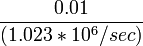$\frac {0.01} {(1.023*10^6/sec)}$ , or approximately 10 nanoseconds for the C/A code. Since GPS signals propagate at the speed of light, this represents an error of about 3 meters.

This component of position accuracy can be improved by a factor of 10 using the higher-chiprate P(Y) signal. Assuming the same one percent of bit pulse width accuracy, the high-frequency P(Y) signal results in an accuracy of $\frac {(0.01*300,000,000 \ m/sec)} {(10.23*10^6/sec)}$ or about 30 centimeters.

[edit] Atmospheric effects

Inconsistencies of atmospheric conditions affect the speed of the GPS signals as they pass through the Earth's atmosphere, especially the ionosphere. Correcting these errors is a significant challenge to improving GPS position accuracy. These effects are smallest when the satellite is directly overhead and become greater for satellites nearer the horizon since the path through the atmosphere is longer (see airmass). Once the receiver's approximate location is known, a mathematical model can be used to estimate and compensate for these errors.

Because ionospheric delay affects the speed of microwave signals differently depending on their frequency — a characteristic known as dispersion - delays measured on two or more frequency bands can be used to measure dispersion, and this measurement can then be used to estimate the delay at each frequency.^[51] Some military and expensive survey-grade civilian receivers measure the different delays in the L1 and L2 frequencies to measure atmospheric dispersion, and apply a more precise correction. This can be done in civilian receivers without decrypting the P(Y) signal carried on L2, by tracking the carrier wave instead of the modulated code. To facilitate this on lower cost receivers, a new civilian code signal on L2, called L2C, was added to the Block IIR-M satellites, which was first launched in 2005. It allows a direct comparison of the L1 and L2 signals using the coded signal instead of the carrier wave. (see Atmospheric Effects in "Sources of Errors in GPS")

The effects of the ionosphere generally change slowly, and can be averaged over time. The effects for any particular geographical area can be easily calculated by comparing the GPS-measured position to a known surveyed location. This correction is also valid for other receivers in the same general location. Several systems send this information over radio or other links to allow L1-only receivers to make ionospheric corrections. The ionospheric data are transmitted via satellite in Satellite Based Augmentation Systems (SBAS) such as WAAS (available in North America and Hawaii), EGNOS (Europe and Asia) or MSAS (Japan), which transmits it on the GPS frequency using a special pseudo-random noise sequence (PRN), so only one receiver and antenna are required.

Humidity also causes a variable delay, resulting in errors similar to ionospheric delay, but occurring in the troposphere. This effect both is more localized and changes more quickly than ionospheric effects, and is not frequency dependent. These traits make precise measurement and compensation of humidity errors more difficult than ionospheric effects.^{[citation needed]}

Changes in receiver altitude also change the amount of delay, due to the signal passing through less of the atmosphere at higher elevations. Since the GPS receiver computes its approximate altitude, this error is relatively simple to correct, either by applying a function regression or correlating margin of atmospheric error to ambient pressure using a barometric altimeter.^{[citation needed]}

[edit] Multipath effects

GPS signals can also be affected by multipath issues, where the radio signals reflect off surrounding terrain; buildings, canyon walls, hard ground, etc. These delayed signals can cause inaccuracy. A variety of techniques, most notably narrow correlator spacing, have been developed to mitigate multipath errors. For long delay multipath, the receiver itself can recognize the wayward signal and discard it. To address shorter delay multipath from the signal reflecting off the ground, specialized antennas (e.g. a choke ring antenna) may be used to reduce the signal power as received by the antenna. Short delay reflections are harder to filter out because they interfere with the true signal, causing effects almost indistinguishable from routine fluctuations in atmospheric delay.

Multipath effects are much less severe in moving vehicles. When the GPS antenna is moving, the false solutions using reflected signals quickly fail to converge and only the direct signals result in stable solutions.

[edit] Ephemeris and clock errors

While the ephemeris data is transmitted every 30 seconds, the information itself may be up to two hours old. Data up to four hours old is considered valid for calculating positions, but may not indicate the satellite's actual position. If a fast Time To First Fix (TTFF) is needed, it is possible to upload a valid ephemeris to a receiver, and in addition to setting the time, a position fix can be obtained in under ten seconds. It is feasible to put such ephemeris data on the web so it can be loaded into mobile GPS devices.^[52] See also Assisted GPS.

The satellite's atomic clocks experience noise and clock drift errors. The navigation message contains corrections for these errors and estimates of the accuracy of the atomic clock. However, they are based on observations and may not indicate the clock's current state.

These problems tend to be very small, but may add up to a few meters (10s of feet) of inaccuracy.^[53]

[edit] Geometric dilution of precision computation (DOP)

As a first step in computing DOP, consider the unit vector from the receiver to satellite i with components,

$\frac {(x_i- x)} {R_i}, \frac {(y_i-y)} {R_i}, and \frac {(z_i-z)} {R_i}$ where the distance from receiver to the satellite, $\ R_i$ , is given by

$R_i= \sqrt{(x_i- x)^2 + (y_i-y)^2 + (z_i-z)^2}$ and where $\ x, y, and\ z$ denote the position of the receiver and $\ x_i, y_i, and\ z_i$ denote the position of satellite i. Formulate the matrix A as

$A = \begin{bmatrix} \frac {(x_1- x)} {R_1} & \frac {(y_1-y)} {R_1} & \frac {(z_1-z)} {R_1} & c \\ \frac {(x_2- x)} {R_2} & \frac {(y_2-y)} {R_2} & \frac {(z_2-z)} {R_2} & c \\ \frac {(x_3- x)} {R_3} & \frac {(y_3-y)} {R_3} & \frac {(z_3-z)} {R_3} & c \\ \frac {(x_4- x)} {R_4} & \frac {(y_4-y)} {R_4} & \frac {(z_4-z)} {R_4} & c \end{bmatrix}$

The first three elements of each row of A are the components of a unit vector from the receiver to the indicated satellite. The elements in the fourth column are c where c denotes the speed of light. Formulate the matrix, Q, as

$Q = \left (A^T A \right )^{-1}$

This computation is in accordance with "Section 1.4.2 of PRINCIPLES OF SATELLITE POSITIONING" where the weighting matrix, P, has been set to the identity matrix.

The elements of the Q matrix are designated as

$Q = \begin{bmatrix} d_x^2 & d_{xy}^2 & d_{xz}^2 & d_{xt}^2 \\ d_{xy}^2 & d_{y}^2 & d_{yz}^2 & d_{yt}^2 \\ d_{xz}^2 & d_{yz}^2 & d_{z}^2 & d_{zt}^2 \\ d_{xt}^2 & d_{yt}^2 & d_{zt}^2 & d_{t}^2 \end{bmatrix}$

The Greek letter $\ \sigma$ is used quite often where we have used d. However the elements of the Q matrix do not represent variances and covariances as they are defined in probability and statistics. Instead they are strictly geometric terms. Therefore d as in dilution of precision is used. PDOP, TDOP and GDOP are given by

$PDOP = \sqrt{d_x^2 + d_y^2 + d_z^2}$ ,

$\ TDOP = \sqrt{d_{t}^2}$ , and

$GDOP = \sqrt{PDOP^2 + TDOP^2}$ in agreement with "Section 1.4.9 of PRINCIPLES OF SATELLITE POSITIONING".

The horizontal dilution of precision, 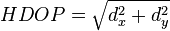$HDOP = \sqrt{d_x^2 + d_y^2}$ , and the vertical dilution of precision, $\ VDOP = \sqrt{d_{z}^2}$ , are both dependent on the coordinate system used. To correspond to the local horizon plane and the local vertical, x, y, and z should denote positions in either a North, East, Down coordinate system or a South, East, Up coordinate system.

[edit] Derivation of DOP Equations

The equations for computing the geometric dilution of precision terms have been described in the previous section. This section describes the derivation of these equations. The method used here is similar to that used in "Global Positioning System (preview) by Parkinson and Spiker"

Consider the position error vector, e, defined as the vector from the intersection of the four sphere surfaces corresponding to the pseudoranges to the true position of the receiver. 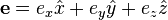$\mathbf{e} = e_x\hat{x} + e_y\hat{y} + e_z\hat{z}$ where bold denotes a vector and 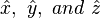$\hat{x},\ \hat{y},\ and\ \hat{z}$ denote unit vectors along the x, y, and z axes respectively. Let $\ e_t$ denote the time error, the true time minus the receiver indicated time. Assume that the mean value of the three components of e and $\ e_t$ are zero.

$A\ \begin{bmatrix} e_x \\ e_y \\ e_z \\ e_t \end{bmatrix} = \begin{bmatrix} \frac {(x_1- x)} {R_1} & \frac {(y_1-y)} {R_1} & \frac {(z_1-z)} {R_1} & c \\ \frac {(x_2- x)} {R_2} & \frac {(y_2-y)} {R_2} & \frac {(z_2-z)} {R_2} & c \\ \frac {(x_3- x)} {R_3} & \frac {(y_3-y)} {R_3} & \frac {(z_3-z)} {R_3} & c \\ \frac {(x_4- x)} {R_4} & \frac {(y_4-y)} {R_4} & \frac {(z_4-z)} {R_4} & c \end{bmatrix}\ \begin{bmatrix} e_x \\ e_y \\ e_z \\ e_t \end{bmatrix} = \begin{bmatrix} e_1 \\ e_2 \\ e_3 \\ e_4 \end{bmatrix} \ (1)$

where $\ e_1,\ e_2,\ e_3,\ and\ e_4$ are the errors in pseudoranges 1 through 4 respectively. This equation comes from linearizing the equation relating pseudoranges to receiver position, satellite positions, and receiver clock errors as shown in [2] . Multiplying both sides by $\ A^{-1} \$ there results

$\ \begin{bmatrix} e_x \\ e_y \\ e_z \\ e_t \end{bmatrix} = A^{-1} \begin{bmatrix} e_1 \\ e_2 \\ e_3 \\ e_4 \end{bmatrix} \ (2)$ .

Transposing both sides

$\ \begin{bmatrix} e_x & e_y & e_z & e_t \end{bmatrix} = \begin{bmatrix} e_1 & e_2 & e_3 & e_4 \end{bmatrix}\left (A^{-1} \right )^T \ (3)$ .

Post multiplying the matrices on both sides of equation (2) by the corresponding matrices in equation (3), there results

$\ \begin{bmatrix} e_x \\ e_y \\ e_z \\ e_t \end{bmatrix} \begin{bmatrix} e_x & e_y & e_z & e_t \end{bmatrix} = A^{-1} \begin{bmatrix} e_1 \\ e_2 \\ e_3 \\ e_4 \end{bmatrix} \begin{bmatrix} e_1 & e_2 & e_3 & e_4 \end{bmatrix}\left (A^{-1} \right )^T \ (4)$ .

Taking the expected value of both sides and taking the non-random matrices outside the expectation operator, E, there results

$\ E \left (\begin{bmatrix} e_x \\ e_y \\ e_z \\ e_t \end{bmatrix} \begin{bmatrix} e_x & e_y & e_z & e_t \end{bmatrix} \right ) = A^{-1} \ E \left (\begin{bmatrix} e_1 \\ e_2 \\ e_3 \\ e_4 \end{bmatrix} \begin{bmatrix} e_1 & e_2 & e_3 & e_4 \end{bmatrix} \right ) \left (A^{-1} \right )^T \ (5)$ .

Assuming the pseudorange errors are uncorrelated and have the same variance, the covariance matrix on the right side can be expressed as a scalar times the identity matrix. Thus

$\begin{bmatrix} \sigma_x^2 & \sigma_{xy}^2 & \sigma_{xz}^2 & \sigma_{xt}^2 \\ \sigma_{xy}^2 & \sigma_{y}^2 & \sigma_{yz}^2 & \sigma_{yt}^2 \\ \sigma_{xz}^2 & \sigma_{yz}^2 & \sigma_{z}^2 & \sigma_{zt}^2 \\ \sigma_{xt}^2 & \sigma_{yt}^2 & \sigma_{zt}^2 & \sigma_{t}^2 \end{bmatrix} = \sigma_R^2 \ A^{-1} \left (A^{-1} \right )^T = \sigma_R^2 \ \left (A^T A \right )^{-1} \ (6)$

since $\ A^{-1} \left (A^{-1} \right )^T \left (A^T A \right ) = I$

Note: $\left (A^{-1} \right )^T = \left (A^{T} \right )^{-1},\$ since $\ I =\left (A A^{-1} \right )^T = \left (A^{-1} \right )^T A^T$

Substituting for $\left (A^T A \right )^{-1} = Q$ there follows

$\begin{bmatrix} \sigma_x^2 & \sigma_{xy}^2 & \sigma_{xz}^2 & \sigma_{xt}^2 \\ \sigma_{xy}^2 & \sigma_{y}^2 & \sigma_{yz}^2 & \sigma_{yt}^2 \\ \sigma_{xz}^2 & \sigma_{yz}^2 & \sigma_{z}^2 & \sigma_{zt}^2 \\ \sigma_{xt}^2 & \sigma_{yt}^2 & \sigma_{zt}^2 & \sigma_{t}^2 \end{bmatrix} = \sigma_R^2 \ \begin{bmatrix} d_x^2 & d_{xy}^2 & d_{xz}^2 & d_{xt}^2 \\ d_{xy}^2 & d_{y}^2 & d_{yz}^2 & d_{yt}^2 \\ d_{xz}^2 & d_{yz}^2 & d_{z}^2 & d_{zt}^2 \\ d_{xt}^2 & d_{yt}^2 & d_{zt}^2 & d_{t}^2 \end{bmatrix} \ (7)$

From equation (7), it follows that the variances of indicated receiver position and time are

$\sigma_{rc}^2 = \sigma_x^2 + \sigma_y^2 + \sigma_z^2 = \sigma_R^2 \left (d_x^2 + d_y^2 + d_z^2 \right ) = PDOP^2 \sigma_R^2$ and

$\sigma_t^2 = \sigma_R^2 d_t^2 = TDOP^2 \sigma_R^2$ .

The remaining position and time error variance terms follow in a straightforward manner.

[edit] Selective availability

GPS includes a (currently disabled) feature called Selective Availability (SA) that adds intentional, time varying errors of up to 100 meters (328 ft) to the publicly available navigation signals. This was intended to deny an enemy the use of civilian GPS receivers for precision weapon guidance.

SA errors are actually pseudorandom, generated by a cryptographic algorithm from a classified seed key available only to authorized users (the US military, its allies and a few other users, mostly government) with a special military GPS receiver. Mere possession of the receiver is insufficient; it still needs the tightly controlled daily key.

Before it was turned off in 2000, typical SA errors were 10 meters (32 ft) horizontally and 30 meters (98 ft) vertically. Because SA affects every GPS receiver in a given area almost equally, a fixed station with an accurately known position can measure the SA error values and transmit them to the local GPS receivers so they may correct their position fixes. This is called Differential GPS or DGPS. DGPS also corrects for several other important sources of GPS errors, particularly ionospheric delay, so it continues to be widely used even though SA has been turned off. The ineffectiveness of SA in the face of widely available DGPS was a common argument for turning off SA, and this was finally done by order of President Clinton in 2000.

Another restriction on GPS, antispoofing, remains on. This encrypts the P-code so that it cannot be mimicked by an enemy transmitter sending false information. Few civilian receivers have ever used the P-code, and the accuracy attainable with the public C/A code is so much better than originally expected (especially with DGPS) that the antispoof policy has relatively little effect on most civilian users. Turning off antispoof would primarily benefit surveyors and some scientists who need extremely precise positions for experiments such as tracking the motion of a tectonic plate.

DGPS services are widely available from both commercial and government sources. The latter include WAAS and the US Coast Guard's network of LF marine navigation beacons. The accuracy of the corrections depends on the distance between the user and the DGPS receiver. As the distance increases, the errors at the two sites will not correlate as well, resulting in less precise differential corrections.

During the 1990-91 Gulf War, the shortage of military GPS units caused many troops and their families to buy readily available civilian units. This significantly impeded the US military's own battlefield use of GPS, so the military made the decision to turn off SA for the duration of the war.

In the 1990s, the FAA started pressuring the military to turn off SA permanently. This would save the FAA millions of dollars every year in maintenance of their own radio navigation systems. The amount of error added was "set to zero"^[54] at midnight on May 1, 2000 following an announcement by U.S. President Bill Clinton, allowing users access to the error-free L1 signal. Per the directive, the induced error of SA was changed to add no error to the public signals (C/A code). Clinton's executive order required SA to be set to zero by 2006; it happened in 2000 once the US military developed a new system that provides the ability to deny GPS (and other navigation services) to hostile forces in a specific area of crisis without affecting the rest of the world or its own military systems.^[54]

Selective Availability is still a system capability of GPS, and error could, in theory, be reintroduced at any time. In practice, in view of the hazards and costs this would induce for US and foreign shipping, it is unlikely to be reintroduced, and various government agencies, including the FAA,^[55] have stated that it is not intended to be reintroduced.

One interesting side effect of the Selective Availability hardware is the capability to correct the frequency of the GPS cesium and rubidium atomic clocks to an accuracy of approximately 2 × 10^-13 (one in five trillion). This represented a significant improvement over the raw accuracy of the clocks.^{[citation needed]}

On 19 September 2007, the United States Department of Defense announced that future GPS III satellites will not be capable of implementing SA,^[56] eventually making the policy permanent.^[57]

[edit] Relativity

Satellite clocks are slowed by their orbital speed but sped up by their distance out of the Earth's gravitational well.

According to the theory of relativity, due to their constant movement and height relative to the Earth-centered inertial reference frame, the clocks on the satellites are affected by their speed (special relativity) as well as their gravitational potential (general relativity). For the GPS satellites, general relativity predicts that the atomic clocks at GPS orbital altitudes will tick more rapidly, by about 45.9 microseconds (μs) per day, because they have a higher gravitational potential than atomic clocks on Earth's surface. Special relativity predicts that atomic clocks moving at GPS orbital speeds will tick more slowly than stationary ground clocks by about 7.2 μs per day. When combined, the discrepancy is about 38 microseconds per day; a difference of 4.465 parts in 10¹⁰.^[58] To account for this, the frequency standard on board each satellite is given a rate offset prior to launch, making it run slightly slower than the desired frequency on Earth; specifically, at 10.22999999543 MHz instead of 10.23 MHz.^[59] Since the atomic clocks on board the GPS satellites are precisely tuned, it makes the system a practical engineering application of the scientific theory of relativity in a real-world environment. Placing atomic clocks on artificial satellites to test Einstein's general theory was first proposed by Friedwardt Winterberg in 1955.^[60]

[edit] Sagnac distortion

GPS observation processing must also compensate for the Sagnac effect. The GPS time scale is defined in an inertial system but observations are processed in an Earth-centered, Earth-fixed (co-rotating) system, a system in which simultaneity is not uniquely defined. A Lorentz transformation is thus applied to convert from the inertial system to the ECEF system. The resulting signal run time correction has opposite algebraic signs for satellites in the Eastern and Western celestial hemispheres. Ignoring this effect will produce an east-west error on the order of hundreds of nanoseconds, or tens of meters in position.^[61]

[edit] Possible Sources of Interference

[edit] Natural sources

Since GPS signals at terrestrial receivers tend to be relatively weak, natural radio signals or scattering of the GPS signals can desensitize the receiver, making acquiring and tracking the satellite signals difficult or impossible.

Space weather degrades GPS operation in two ways, direct interference by solar radio burst noise in the same frequency band ^[62] or by scattering of the GPS radio signal in ionospheric irregularities referred to as scintillation ^[63]. Both forms of degradation follow the 11 year solar cycle and are a maximum at sunspot maximum although they can occur at anytime. Solar radio bursts are associated with solar flares and their impact can affect reception over the half of the Earth facing the sun. Scintillation occurs most frequently at tropical latitudes where it is a night time phenomenon. It occurs less frequently at high latitudes or mid-latitudes where magnetic storms can lead to scintillation ^[64]. In addition to producing scintillation, magnetic storms can produce strong ionospheric gradients that degrade the accuracy of SBAS systems ^[65].

[edit] Artificial sources

In automotive GPS receivers, metallic features in windshields,^[66] such as defrosters, or car window tinting films^[67] can act as a Faraday cage, degrading reception just inside the car.

Man-made EMI (electromagnetic interference) can also disrupt, or jam, GPS signals. In one well documented case, the entire harbor of Moss Landing, California was unable to receive GPS signals due to unintentional jamming caused by malfunctioning TV antenna preamplifiers.^[68]^[69] Intentional jamming is also possible. Generally, stronger signals can interfere with GPS receivers when they are within radio range, or line of sight. In 2002, a detailed description of how to build a short range GPS L1 C/A jammer was published in the online magazine Phrack.^[70]

The U.S. government believes that such jammers were used occasionally during the 2001 war in Afghanistan and the U.S. military claimed to destroy six GPS jammers during the Iraq War, including one that was destroyed ironically with a GPS-guided bomb.^[71] Such a jammer is relatively easy to detect and locate, making it an attractive target for anti-radiation missiles. The UK Ministry of Defence tested a jamming system in the UK's West Country on 7 and 8 June 2007.^[72]

Some countries allow the use of GPS repeaters to allow for the reception of GPS signals indoors and in obscured locations, however, under EU and UK laws, the use of these is prohibited as the signals can cause interference to other GPS receivers that may receive data from both GPS satellites and the repeater.

Due to the potential for both natural and man-made noise, numerous techniques continue to be developed to deal with the interference. The first is to not rely on GPS as a sole source. According to John Ruley, "IFR pilots should have a fallback plan in case of a GPS malfunction".^[73] Receiver Autonomous Integrity Monitoring (RAIM) is a feature now included in some receivers, which is designed to provide a warning to the user if jamming or another problem is detected. The U.S. military has also deployed their Selective Availability / Anti-Spoofing Module (SAASM) in the Defense Advanced GPS Receiver (DAGR). In demonstration videos, the DAGR is able to detect jamming and maintain its lock on the encrypted GPS signals during interference which causes civilian receivers to lose lock.^[74]

[edit] Accuracy enhancement

[edit] Augmentation

Main article: GNSS Augmentation

Augmentation methods of improving accuracy rely on external information being integrated into the calculation process. There are many such systems in place and they are generally named or described based on how the GPS sensor receives the information. Some systems transmit additional information about sources of error (such as clock drift, ephemeris, or ionospheric delay), others provide direct measurements of how much the signal was off in the past, while a third group provide additional navigational or vehicle information to be integrated in the calculation process.

Examples of augmentation systems include the Wide Area Augmentation System, Differential GPS, Inertial Navigation Systems and Assisted GPS.

[edit] Precise monitoring

The accuracy of a calculation can also be improved through precise monitoring and measuring of the existing GPS signals in additional or alternate ways.

After SA, which has been turned off, the largest error in GPS is usually the unpredictable delay through the ionosphere. The spacecraft broadcast ionospheric model parameters, but errors remain. This is one reason the GPS spacecraft transmit on at least two frequencies, L1 and L2. Ionospheric delay is a well-defined function of frequency and the total electron content (TEC) along the path, so measuring the arrival time difference between the frequencies determines TEC and thus the precise ionospheric delay at each frequency.

Receivers with decryption keys can decode the P(Y)-code transmitted on both L1 and L2. However, these keys are reserved for the military and "authorized" agencies and are not available to the public. Without keys, it is still possible to use a codeless technique to compare the P(Y) codes on L1 and L2 to gain much of the same error information. However, this technique is slow, so it is currently limited to specialized surveying equipment. In the future, additional civilian codes are expected to be transmitted on the L2 and L5 frequencies (see GPS modernization, below). Then all users will be able to perform dual-frequency measurements and directly compute ionospheric delay errors.

A second form of precise monitoring is called Carrier-Phase Enhancement (CPGPS). The error, which this corrects, arises because the pulse transition of the PRN is not instantaneous, and thus the correlation (satellite-receiver sequence matching) operation is imperfect. The CPGPS approach utilizes the L1 carrier wave, which has a period one one-thousandth of the C/A bit period, to act as an additional clock signal and resolve the uncertainty. The phase difference error in the normal GPS amounts to between 2 and 3 meters (6 to 10 ft) of ambiguity. CPGPS working to within 1% of perfect transition reduces this error to 3 centimeters (1 inch) of ambiguity. By eliminating this source of error, CPGPS coupled with DGPS normally realizes between 20 and 30 centimeters (8 to 12 inches) of absolute accuracy.

Relative Kinematic Positioning (RKP) is another approach for a precise GPS-based positioning system. In this approach, determination of range signal can be resolved to a precision of less than 10 centimeters (4 in). This is done by resolving the number of cycles in which the signal is transmitted and received by the receiver. This can be accomplished by using a combination of differential GPS (DGPS) correction data, transmitting GPS signal phase information and ambiguity resolution techniques via statistical tests—possibly with processing in real-time (real-time kinematic positioning, RTK).

[edit] Timekeeping

While most clocks are synchronized to Coordinated Universal Time (UTC), the atomic clocks on the satellites are set to GPS time. The difference is that GPS time is not corrected to match the rotation of the Earth, so it does not contain leap seconds or other corrections which are periodically added to UTC. GPS time was set to match Coordinated Universal Time (UTC) in 1980, but has since diverged. The lack of corrections means that GPS time remains at a constant offset (TAI - GPS = 19 seconds) with International Atomic Time (TAI). Periodic corrections are performed on the on-board clocks to correct relativistic effects and keep them synchronized with ground clocks.

The GPS navigation message includes the difference between GPS time and UTC, which as of 2009 is 15 seconds due to the leap second added to UTC December 31 2008. Receivers subtract this offset from GPS time to calculate UTC and specific timezone values. New GPS units may not show the correct UTC time until after receiving the UTC offset message. The GPS-UTC offset field can accommodate 255 leap seconds (eight bits) which, given the current rate of change of the Earth's rotation (with one leap second introduced approximately every 18 months), should be sufficient to last until approximately year 2300.

As opposed to the year, month, and day format of the Gregorian calendar, the GPS date is expressed as a week number and a day-of-week number. The week number is transmitted as a ten-bit field in the C/A and P(Y) navigation messages, and so it becomes zero again every 1,024 weeks (19.6 years). GPS week zero started at 00:00:00 UTC (00:00:19 TAI) on January 6 1980, and the week number became zero again for the first time at 23:59:47 UTC on August 21 1999 (00:00:19 TAI on August 22 1999). To determine the current Gregorian date, a GPS receiver must be provided with the approximate date (to within 3,584 days) to correctly translate the GPS date signal. To address this concern the modernized GPS navigation message uses a 13-bit field, which only repeats every 8,192 weeks (157 years), thus lasting until year 2137 (157 years after GPS week zero).

[edit] Modernization

Main article: GPS modernization

Having reached the program's requirements for Full Operational Capability (FOC) on July 17, 1995,^[75] the GPS completed its original design goals. However, additional advances in technology and new demands on the existing system led to the effort to modernize the GPS. Announcements from the U.S. Vice President and the White House in 1998 initiated these changes, and in 2000 the U.S. Congress authorized the effort, referring to it as GPS III.

The project aims to improve the accuracy and availability for all users and involves a new control segment (called GPS OCX), new ground stations, new satellites, and four additional navigation signals. New civilian signals are called L2C, L5 and L1C; the new military code is called M-Code. Initial Operational Capability (IOC) of the L2C code is expected in 2008.^[76] A goal of 2013 has been established for the entire program, with incentives offered to the contractors if they can complete it by 2011 (See GPS signals).

[edit] Applications

The Global Positioning System, while originally a military project, is considered a dual-use technology, meaning it has significant applications for both the military and the civilian industry.

[edit] Military

The military applications of GPS span many purposes:

Navigation: GPS allows soldiers to find objectives in the dark or in unfamiliar territory, and to coordinate the movement of troops and supplies. The GPS-receivers that commanders and soldiers use are respectively called the Commanders Digital Assistant and the Soldier Digital Assistant.^[77]^[78]^[79]^[80]
Target tracking: Various military weapons systems use GPS to track potential ground and air targets before they are flagged as hostile.^{[citation needed]} These weapon systems pass GPS co-ordinates of targets to precision-guided munitions to allow them to engage the targets accurately. Military aircraft, particularly those used in air-to-ground roles use GPS to find targets (for example, gun camera video from AH-1 Cobras in Iraq show GPS co-ordinates that can be looked up in Google Earth^{[citation needed]}).
Missile and projectile guidance: GPS allows accurate targeting of various military weapons including ICBMs, cruise missiles and precision-guided munitions. Artillery projectiles with embedded GPS receivers able to withstand accelerations of 12,000G have been developed for use in 155 mm howitzers.^[81]
Search and Rescue: Downed pilots can be located faster if they have a GPS receiver.
Reconnaissance and Map Creation: The military use GPS extensively to aid mapping and reconnaissance.
The GPS satellites also carry a set of nuclear detonation detectors consisting of an optical sensor (Y-sensor), an X-ray sensor, a dosimeter, and an Electro-Magnetic Pulse (EMP) sensor (W-sensor) which form a major portion of the United States Nuclear Detonation Detection System.^[82]^[83]

[edit] Civilian

This antenna is mounted on the roof of a hut containing a scientific experiment needing precise timing.

Many civilian applications benefit from GPS signals, using one or more of three basic components of the GPS: absolute location, relative movement, and time transfer.

The ability to determine the receiver's absolute location allows GPS receivers to perform as a surveying tool or as an aid to navigation. The capacity to determine relative movement enables a receiver to calculate local velocity and orientation, useful in vessels or observations of the Earth. Being able to synchronize clocks to exacting standards enables time transfer, which is critical in large communication and observation systems. An example is CDMA digital cellular. Each base station has a GPS timing receiver to synchronize its spreading codes with other base stations to facilitate inter-cell hand off and support hybrid GPS/CDMA positioning of mobiles for emergency calls and other applications. Finally, GPS enables researchers to explore the Earth environment including the atmosphere, ionosphere and gravity field. GPS survey equipment has revolutionized tectonics by directly measuring the motion of faults in earthquakes.

The US Government controls the export of some civilian receivers. All GPS receivers capable of functioning above 18 km (60,000 ft) altitude and 515 m/s (1,000 knots) ^[84] are classified as munitions (weapons) for which US State Department export licenses are required. These parameters are clearly chosen to prevent use of a receiver in a ballistic missile. It would not prevent use in a cruise missile since their altitudes and speeds are similar to those of ordinary aircraft.

This rule applies even to otherwise purely civilian units that only receive the L1 frequency and the C/A code and cannot correct for SA, etc.

Disabling operation above these limits exempts the receiver from classification as a munition. Different vendors have interpreted these limitations differently. The rule specifies operation above 18km and 515 m/s, but some receivers stop operating at 18km even when stationary. This has caused problems with some amateur radio balloon launches as they regularly reach 100,000 feet (30km).

GPS tours are also an example of civilian use. The GPS is used to determine which content to display. For instance, when approaching a monument it would tell you about the monument.

GPS functionality has now started to move into mobile phones en masse. The first handsets with integrated GPS were launched already in the late 1990’s, and were available for broader consumer availability on networks such as those run by Nextel, Sprint and Verizon in 2002 in response to US FCC mandates for handset positioning in emergency calls. Capabilities for access by third party software developers to these features were slower in coming, with Nextel opening up those APIs upon launch to any developer, Sprint following in 2006, and Verizon soon thereafter.

[edit] Awards

Two GPS developers received the National Academy of Engineering Charles Stark Draper Prize for 2003:

Ivan Getting, emeritus president of The Aerospace Corporation and engineer at the Massachusetts Institute of Technology, established the basis for GPS, improving on the World War II land-based radio system called LORAN (Long-range Radio Aid to Navigation).
Bradford Parkinson, professor of aeronautics and astronautics at Stanford University, conceived the present satellite-based system in the early 1960s and developed it in conjunction with the U.S. Air Force.

One GPS developer, Roger L. Easton, received the National Medal of Technology on February 13, 2006 at the White House.^[85]

On February 10, 1993, the National Aeronautic Association selected the Global Positioning System Team as winners of the 1992 Robert J. Collier Trophy, the most prestigious aviation award in the United States. This team consists of researchers from the Naval Research Laboratory, the U.S. Air Force, the Aerospace Corporation, Rockwell International Corporation, and IBM Federal Systems Company. The citation accompanying the presentation of the trophy honors the GPS Team "for the most significant development for safe and efficient navigation and surveillance of air and spacecraft since the introduction of radio navigation 50 years ago."

[edit] Other systems

Main article: Global Navigation Satellite System

Other satellite navigation systems in use or various states of development include:

Beidou – China's regional system that China has proposed to expand into a global system named COMPASS.
Galileo – a proposed global system being developed by the European Union, joined by China, Israel, India, Morocco, Saudi Arabia, South Korea, and Ukraine, planned to be operational by 2013.
GLONASS – Russia's global system which is being restored to full availability in partnership with India.
Indian Regional Navigational Satellite System (IRNSS) – India's proposed regional system.
QZSS – Japanese proposed regional system, adding better coverage to the Japanese Islands.

[edit] Multidimensional Newton-Raphson for GPS

This section provides a more detailed discussion of the equations used in the second method described in Position calculation advanced. The linearized equations are developed using the appropriate partial derivatives and the algorithm is described. In ^[43] the same method is discussed but the equations are not shown. Let $x, y\;$ and $z\;$ denote the true coordinates of GPS receiver position at time, $\ t$ . Let $\ b$ denote the unknown clock error or bias, the amount by which the receiver's clock is slow. Let the coordinates of each satellite, and the time the message was sent, be $\left [x_i, y_i, z_i, t_i\right ]$ , let the GPS clock's indicated received time be $tr_i\; \mbox{for} \ i=1,2,3,4$ and c be the speed of light. The pseudorange is computed as $p_i = \left (tr_i - t_i \right )c$ . Assume the message travels at the speed of light, then the pseudorange satisfies the equation,

$p_i = \sqrt{(x-x_i)^2 + (y-y_i)^2 + (z-z_i)^2}- bc, \;\; \mbox{for} \; i=1,2,3,4. \qquad (1)$

When an approximate solution, $\left [x^{(k)}, y^{(k)}, z^{(k)}, b^{(k)}\right ]$ rather than the exact solution, $\left [x, y, z, b\right ]$ is used in equation 1, there is a residual, $f_i^{(k)}$ . Transforming $\ p_i$ to the right hand side of the equation there results,

$f_i^{(k)} = \sqrt{(x^{(k)}-x_i)^2 + (y^{(k)}-y_i)^2 + (z^{(k)}-z_i)^2}- b^{(k)}c - p_i, \;\; \mbox{for} \; i=1,2,3,4. \qquad (2)$

A solution will have been found when $f_i^{(k)}$ is zero or sufficiently close to zero for $\ i=1,2,3,4$ .

In order to linearize equation 2, the partial derivatives are computed as

$\frac{\partial f_i^{(k)}} {\partial x^{(k)}} = \frac {(x^{(k)} - x_i)} {R_i^{(k)} }, \frac{\partial f_i^{(k)}} {\partial y^{(k)}} = \frac {(y^{(k)}-y_i)} {R_i^{(k)}}, \frac{\partial f_i^{(k)}} {\partial z^{(k)}} = \frac {(z^{(k)} -z_i)} {R_i^{(k)} }, \frac{\partial f_i^{(k)}} {\partial b^{(k)}} = -c \qquad (3)$

where

$R_i^{(k)} = \sqrt{(x^{(k)}-x_i)^2 + (y^{(k)}-y_i)^2 + (z^{(k)}-z_i)^2}$ .

Linearizing the right hand side of equation 2 about the approximate solution, $\left [x^{(k)}, y^{(k)}, z^{(k)}, b^{(k)}\right ]$ there results

$f_i^{(k)} = \frac {(x^{(k)}-x_i)} {R_i^{(k)}} x^{(k)} + \frac {(y^{(k)}-y_i)} {R_i^{(k)}} y^{(k)} + \frac {(z^{(k)}-z_i)} {R_i^{(k)}} z^{(k)} - b^{(k)}c - p_i + \epsilon_i \;\; \mbox{for} \; i=1,2,3,4 \qquad (4)$

where $\ \epsilon_i$ is the residual due to linearization which is in addition to the residual, $f_i^{(k)}$ , due to an approximate solution.

In order to drive $f_i^{(k+1)}$ closer to zero choose the values $\left [x^{(k+1)}, y^{(k+1)}, z^{(k+1)}, b^{(k+1)}\right ]$ such that

$- f_i^{(k)} = \frac {(x^{(k)}-x_i)} {p_i} (x^{(k+1)}- x^{(k)}) + \frac {(y^{(k)}-y_i)} {p_i} (y^{(k+1)}- y^{(k)})\;+$ $\frac {(z^{(k)}-z_i)} {p_i} (z^{(k+1)}- z^{(k)}) - (b^{(k+1)} - b^{(k)})c - p_i. \qquad (5)$

That is choose the values

$\left [x^{(k+1)}, y^{(k+1)}, z^{(k+1)}, b^{(k+1)}\right ]$

such that the residual in equation 2 changes by approximately $\ - f_i^{(k)}$ .

Let

$\Delta x^{(k+1)}\ =\ (x^{(k+1)}- x^{(k)}),\ \Delta y^{(k+1)}\ =\ (y^{(k+1)}- y^{(k)}),\ \Delta z^{(k+1)}\ =\ (z^{(k+1)}- z^{(k)}),$

and $\ \Delta b^{(k+1)}\ =\ (b^{(k+1)}- b^{(k)}).$

Substituting and transposing $\ p_i$ to the left hand side of the equation, there results

$- f_i^{(k)} + p_i = \frac {(x^{(k)}-x_i)} {p_i} \Delta x^{(k+1)} + \frac {(y^{(k)}-y_i)} {p_i} \Delta y^{(k+1)} \;+$ $\frac {(z^{(k)}-z_i)} {p_i} \Delta z^{(k+1)} - \Delta b^{(k+1)} c. \qquad (6)$

Equations 6 provide a set of four linear equations in four unknowns, the delta terms. They are in a form for solution. Using the values of $\; \Delta x^{(k+1)}, \Delta y^{(k+1)}, \Delta z^{(k+1)}$ and $\; \Delta b^{(k+1)}$ determined by this linear equation solution,

$\left [x^{(k+1)}, y^{(k+1)}, z^{(k+1)}, b^{(k+1)}\right ]$

is evaluated using

$x^{(k+1)}\ =\ x^{(k)}\ +\ \Delta x^{(k+1)}, y^{(k+1)}\ =\ y^{(k)}\ +\ \Delta y^{(k+1)}, z^{(k+1)}\ =\ z^{(k)}\ +\ \Delta z^{(k+1)},$

and $b^{(k+1)}\ =\ b^{(k)}\ +\ \Delta b^{(k+1)}. \qquad (7)$

Then set $\ k = k + 1$ in equations 2 through 6, plug the terms

$\left \{ x^{(k+1)}, y^{(k+1)}, z^{(k+1)}, b^{(k+1)} \right \}$

from equations 7 into equations 2, set $\ k = k + 1$ in equations 7, and reevaluate the residuals in equations 2. This procedure is repeated until the residuals are sufficiently small in magnitude.

[edit] See also

Nautical portal

Assisted GPS (A-GPS)
Automotive navigation system
Bluetooth
The American Practical Navigator - Chapter 11 Satellite Navigation
Degree Confluence Project - use GPS to visit integral degrees of latitude and longitude
Exif - GPS data transfer format
Geocaching
Geotagging
GPS drawing
GPS navigation software
GPS signals
GPS tracking
GPS/INS
GPX (data transfer) - XML schema for interchange of waypoints
GSM localization
Height Modernization
High Sensitivity GPS
ID Sniper rifle
List of inventions by the military that are now in mass use
LORAN
Next Generation Air Transportation System
OpenStreetMap - free content maps and street pictures
Plate Boundary Observatory
Point of interest
Radio navigation
RAIM
SIGI
Skyhook Wireless - Wi-Fi Positioning System
Telematics - many telematics devices use GPS to determine the location of mobile equipment
Trilateration

[edit] References

^ Steven R. Strom. "Charting a Course Toward Global Navigation". The Aerospace Corporation. http://www.aero.org/publications/crosslink/summer2002/01.html. Retrieved on 2008-06-27.
^ What does NAVSTAR stand for?
^ "ICAO COMPLETES FACT-FINDING INVESTIGATION". International Civil Aviation Organization. http://www.icao.int/cgi/goto_m.pl?icao/en/trivia/kal_flight_007.htm. Retrieved on 2008-09-15.
^ "History of GPS". usinfo.state.gov. February 3, 2006. http://usinfo.state.gov/xarchives/display.html?p=washfile-english&y=2006&m=February&x=20060203125928lcnirellep0.5061609.
^ Astronautica Acta II, 25 (1956).
^ "United States Naval Observatory ((USNO) - Block II Satellite Information". ftp://tycho.usno.navy.mil/pub/gps/gpsb2.txt.
^ GPS constellation status. Russian Space Agency. April 9, 2008
^ GPS Wing Reaches GPS III IBR Milestone in InsideGNSS November 10, 2008
^ Dietrich Schroeer, Mirco Elena (2000). Technology Transfer. Ashgate. pp. p80. ISBN 075462045X. http://books.google.com/books?lr=&id=I7JRAAAAMAAJ. Retrieved on 2008-05-25.
^ Michael Russell Rip, James M. Hasik (2002). The Precision Revolution: GPS and the Future of Aerial Warfare. Naval Institute Press. ISBN 1557509735. http://books.google.com/books?lr=&id=_wpUAAAAMAAJ. Retrieved on 2008-05-25.
^ United States Department of Defense. Announcement of Initial Operational Capability^{[dead link]} Announcement of Initial Operational Capability at the Internet Archive. December 8, 1993.
^ National Archives and Records Administration. U.S. Global Positioning System Policy. March 29, 1996.
^ 3g.co.uk
^ losangeles.af.mil
^ sidt.gpsworld.com
^ United States Naval Observatory. GPS Constellation Status. Retrieved December 20, 2008.
^ GPS signals travel at the speed of light, so computing the distance for a given elapsed time is almost a straightforward calculation. However, the speed of light varies slightly between the partial vacuum of space and the atmosphere. A receiver can approximate these effects and produce a reasonable estimate. Once a rough position is determined, some receivers carefully compute the amount of atmosphere the signal traveled through and adjust the distance accordingly.
^ Georg zur Bonsen, Daniel Ammann, Michael Ammann, Etienne Favey, Pascal Flammant (2005-04-01). "Continuous Navigation Combining GPS with Sensor-Based Dead Reckoning". GPS World. http://www.gpsworld.com/gpsworld/article/articleDetail.jsp?id=154870&pageID=6.
^ ^a ^b ^c ^d "NAVSTAR GPS USER EQUIPMENT INTRODUCTION" (PDF). US Government. http://www.navcen.uscg.gov/pubs/gps/gpsuser/gpsuser.pdf.
^ "GPS Support Notes" (PDF). January 19, 2007. http://www.navmanwireless.com/uploads/EK/C8/EKC8zb1ITsNwDqWcqLQxiQ/Support_Notes_GPS_OperatingParameters.pdf. Retrieved on 2008-11-10.
^ globalsecurity.org [1].
^ "Navstar GPS and GLONASS: global satellite navigation systems". IEEE. http://ieeexplore.ieee.org/iel1/2219/7072/00285510.pdf?arnumber=285510.
^ Dana, Peter H. (1996-08-08). "GPS Orbital Planes" (GIF). http://www.colorado.edu/geography/gcraft/notes/gps/gif/oplanes.gif.
^ What the Global Positioning System Tells Us about Relativity. Retrieved January 2, 2007.
^ GPS Overview from the NAVSTAR Joint Program Office. Retrieved December 15, 2006.
^ "USCG Navcen: GPS Frequently Asked Questions". http://www.navcen.uscg.gov/faq/gpsfaq.htm. Retrieved on 2007-01-31.
^ Agnew, D.C. and Larson, K.M. (2007). "Finding the repeat times of the GPS constellation". GPS Solutions (Springer) 11 (1): 71--76. doi:10.1007/s10291-006-0038-4. This article from author's web site, with minor correction.
^ Tis-pf-nisws. "Nanu 2008030". http://cgls.uscg.mil/pipermail/gps/2008-March/001625.html.
^ Massatt, Paul; Wayne Brady (Summer 2002). "Optimizing performance through constellation management". Crosslink: 17–21. http://www.aero.org/publications/crosslink/summer2002/index.html.
^ The additional stations are: Washington, DC, England, Argentina, Ecuador, Bahrain and Australia. Source: US Coast Guard General GPS News 9-9-05
^ USNO NAVSTAR Global Positioning System. Retrieved May 14, 2006.
^ Note that though there are many receiver manufacurers, they almost all use one of the chipsets produced for this purpose. An example: "GPS Receiver Chip Performance Survey". GPS Technology Reviews. http://gpstekreviews.com/2007/04/14/gps-receiver-chip-performance-survey/.
^ NMEA NMEA 2000
^ "Publications and Standards from the National Marine Electronics Association (NMEA)". National Marine Electronics Association. http://www.nmea.org/pub/index.html. Retrieved on 2008-06-27.
^ "Interface Specification IS-GPS-200, Revision D: Navstar GPS Space Segment/Navigation User Interfaces" (PDF). Navstar GPS Joint Program Office. http://www.losangeles.af.mil/shared/media/document/AFD-070803-059.pdf. Page 103.
^ How GPS works. Konowa.de (2005).
^ First GPS IIF Satellite Undergoes Environmental Testing. GPS World. November 5, 2007.
^ "[George, M., Hamid, M., and Miller A. Gold Code Generators in Virtex DevicesPDF (126 KB)
^ "GPS - explained (Signals)"
^ "AN02 Network Assistance" (HTML). http://www.navsync.com/notes2.html. Retrieved on 2007-09-10.
^ ^a ^b ^c ^d ^e Press, Flannery, Tekolsky, and Vetterling 1986, Numerical Recipes, The Art of Scientific Computing (Cambridge University Press).
^ Noe, P.S.; Myers, K.A. (March 1976). "A Position Fixing Algorithm for the Low-Cost GPS Receiver". IEEE Transactions on Aerospace and Electronic Systems AES-12 (2): 295–297. doi:10.1109/TAES.1976.308310. http://ieeexplore.ieee.org/xpls/abs_all.jsp?arnumber=4101635.
^ ^a ^b ^c Richard Langley (July/August 1991). "The Mathematics of GPS" (PDF). GPS World. http://gauss.gge.unb.ca/gpsworld/EarlyInnovationColumns/Innov.1991.07-08.pdf.
^ ^a ^b Lundberg, J.B. (2001). "Alternative algorithms for the GPS static positioning solution". Applied Mathematics and Computation (Elsevier) 119 (1): 21--34. doi:10.1016/S0096-3003(99)00219-2.
^ ^a ^b Bancroft, S. (1985). "An Algebraic Solution of the GPS Equations". Aerospace and Electronic Systems, IEEE Transactions on aes-21: 56--59. doi:10.1109/TAES.1985.310538. http://ieeexplore.ieee.org/xpl/freeabs_all.jsp?arnumber=4104017.
^ Jay Farrell, Matthew Barth (1999). The global positioning system and inertial navigation. McGraw-Hill. p. 145. ISBN 007022045X.
^ Krause, L.O. (March 1987). "A Direct Solution to GPS-Type Navigation Equations". Aerospace and Electronic Systems, IEEE Transactions on AES-23 (2): 225–232. doi:10.1109/TAES.1987.313376.
^ ^a ^b Yang Yong and Miao Lingjuan (2004-07-06). "GDOP results in all-in-view positioning and in four optimum satellites positioning with GPS PRN codes ranging". Position Location and Navigation Symposium, 2004. PLANS 2004: 723-727.
^ Peter H. Dana. "Geometric Dilution of Precision (GDOP) and Visibility". University of Colorado at Boulder. http://www.colorado.edu/geography/gcraft/notes/gps/gps.html#Gdop. Retrieved on 2008-07-07.
^ Peter H. Dana. "Receiver Position, Velocity, and Time". University of Colorado at Boulder. http://www.colorado.edu/geography/gcraft/notes/gps/gps.html#PosVelTime. Retrieved on 2008-07-07.
^ The same principle, and the math behind it, can be found in descriptions of pulsar timing by astronomers.
^ Ephemeris Server Example
^ "UNit 1 - Introduction to GPS". http://seismo.berkeley.edu/~battag/GAMITwrkshp/lecturenotes/unit1/unit1.html#3.
^ ^a ^b "Statement by the President regarding the United States' Decision to Stop Degrading Global Positioning System Accuracy". Office of Science and Technology Policy. May 1, 2000. http://www.ngs.noaa.gov/FGCS/info/sans_SA/docs/statement.html. Retrieved on 2009-02-02.
^ "GNSS - Frequently Asked Questions - GPS: Will SA ever be turned back on?". FAA. June 13, 2007. http://www.faa.gov/about/office_org/headquarters_offices/ato/service_units/techops/navservices/gnss/faq/gps/index.cfm#ad3. Retrieved on 2007-12-17.
^ "DoD Permanently Discontinues Procurement Of Global Positioning System Selective Availability". DefenseLink. September 18, 2007. http://www.defenselink.mil/releases/release.aspx?releaseid=11335. Retrieved on 2008-02-20.
^ "Selective Availability". National space-based Positioning, Navigation, and Timing Executive Committee. http://pnt.gov/public/sa/. Retrieved on 2008-02-20.
^ Rizos, Chris. University of New South Wales. GPS Satellite Signals. 1999.
^ The Global Positioning System by Robert A. Nelson Via Satellite, November 1999
^ Astronautica Acta II, 25 (1956).
^ Ashby, Neil Relativity and GPS. Physics Today, May 2002.
^ Cerruti, A., P. M. Kintner, D. E. Gary, A. J. Mannucci, R. F. Meyer, P. H. Doherty, and A. J. Coster (2008), Effect of intense December 2006 solar radio bursts on GPS receivers, Space Weather, doi:10.1029/2007SW000375, October 19, 2008
^ Aarons, Jules and Basu, Santimay, Ionospheric amplitude and phase fluctuations at the GPS frequencies, Proceedings of ION GPS, v 2, 1994, p 1569-1578
^ Ledvina, B. M., J. J. Makela, and P. M. Kintner (2002), First observations of intense GPS L1 amplitude scintillations at midlatitude, Geophys. Res. Lett., 29(14), 1659, doi:10.1029/2002GL014770
^ Tom Diehl, Solar Flares Hit the Earth- WAAS Bends but Does Not Break, SatNav News, volume 23, June 2004
^ "I-PASS Mounting for Vehicles with Special Windshield Features". http://www.illinoistollway.com/pls/portal/docs/PAGE/TW_CONTENT_REPOSITORY/TW_CR_IPASS/LPT-SPECIALWINDSHIELDLIST.PDF.
^ "3M Automotive Films". http://solutions.3m.com/wps/portal/3M/en_US/WF/3MWindowFilms/Products/ProductCatalog/?PC_7_RJH9U5230GE3E02LECFTDQG0V7_nid=9928QS9MGHbeT4DCJBL6BVgl. . Note that the 'Color Stable' films are specifically described as not interfering with satellite signals.
^ The hunt for an unintentional GPS jammer. GPS World. 1 January 2003.
^ EMC compliance club "banana skins" column 222
^ Low Cost and Portable GPS Jammer. Phrack issue 0x3c (60), article 13]. Published December 28, 2002.
^ American Forces Press Service. Centcom charts progress. March 25, 2003.
^ "MoD's tests will send satnav haywire so take a road atlas". The Daily Mail. 2007-06-06. http://www.dailymail.co.uk/news/article-460279/MoDs-tests-send-satnav-haywire-road-atlas.html.
^ Ruley, John. AVweb. GPS jamming. February 12, 2003.
^ Commercial GPS Receivers: Facts for the Warfighter. Hosted at the Joint Chiefs website, linked by the USAF's GPS Wing DAGR program^{[dead link]} website. Accessed on 10 April, 2007
^ US Coast Guard news release. Global Positioning System Fully Operational
^ Hydrographic Society Journal. Developments in Global Navigation Satellite Systems. Issue #104, April 2002. Retrieved April 5, 2007.
^ Commanders Digital Assistant explanation and photo
^ Latest version Commanders Digital Assistant
^ Soldier Digital Assistant explanation and photo
^ Commanders and Soldiers' GPS-receivers
^ "XM982 Excalibur Precision Guided Extended Range Artillery Projectile". GlobalSecurity.org. 2007-05-29. http://www.globalsecurity.org/military/systems/munitions/m982-155.htm. Retrieved on 2007-09-26.
^ Sandia National Laboratory's Nonproliferation programs and arms control technology.
^ Dr. Dennis D. McCrady. "The GPS Burst Detector W-Sensor". Sandia National Laboratories. http://www.osti.gov/bridge/servlets/purl/10176800-S2tU7w/native/10176800.pdf.
^ Arms Control Association.Missile Technology Control Regime. Retrieved May 17, 2006.
^ United States Naval Research Laboratory. National Medal of Technology for GPS. November 21, 2005

[edit] External links

[edit] Government links

GPS.gov — General public education website created by the U.S. Government
National Space-Based PNT Executive Committee—Established in 2004 to oversee management of GPS and GPS augmentations at a national level.
USCG Navigation Center—Status of the GPS constellation, government policy, and links to other references. Also includes satellite almanac data.
Air Force Space Command GPS Operations Center homepage
The GPS Program Office (GPS Wing)—Responsible for designing and acquiring the system on behalf of the US Government.
U.S. Naval Observatory's GPS constellation status
U.S. Army Corps of Engineers manual: NAVSTAR HTML and PDF (22.6 MB, 328 pages)
PNT Selective Availability Announcements
Global Positioning System Systems Engineering Case Study (A detailed history of GPS development)
Federal Aviation Administration's GPS FAQ
National Geodetic Survey Orbits for the Global Positioning System satellites in the Global Navigation Satellite System

[edit] Introductory / tutorial links

GPS Academy Garmin interactive video web site explaing what exactly GPS is and what it can do for you.
Integraph's Geomedia GIS education, GPS dictionary
GPS Basics / u-blox GPS basics tutorial
Differences and Features of handheld GPSs
GPS and GLONASS Simulation(Java applet) Simulation and graphical depiction of space vehicle motion including computation of dilution of precision (DOP)
How does GPS work? TomTom explains GPS, navigation, and digital maps
What is Vehicle Tracking? Chameleon explains GPS' relation to Vehicle Tracking and Vehicle Tracking Systems
How does eGPS work? CSR's online tutorial introduces the concept and principles of enhanced GPS techniques to improve A-GPS performance and provide indoor positioning
Trimble's Online GPS Tutorial Tutorial designed to introduce you to the principles behind GPS
Ted Driver's The Nog Navigation Developer's information and resource site
GPS Satellite Performance

[edit] Technical, historical, and ancillary topics links

The WhereAmI Project — The WhereAmI Project. Personal Location Tracking and Publishing Service.
GPS SPS Performance Standard — The official Standard Positioning Service specification (2008 version).
GPS SPS Performance Standard — The official Standard Positioning Service specification (2001 version).
GPS PPS Performance Standard — The official Precise Positioning Service specification.
Dana, Peter H. "Global Positioning System Overview"
Satellite Navigation: GPS & Galileo (PDF)—16-page paper about the history and working of GPS, touching on the upcoming Galileo
History of GPS, including information about each satellite's configuration and launch.
Chadha, Kanwar. "The Global Positioning System: Challenges in Bringing GPS to Mainstream Consumers" Technical Article (1998)
GPS Weapon Guidance Techniques
RAND history of the GPS (PDF)
GPS-guided educational experience based on the history of a location
GPS Anti-Jam Protection Techniques
Crosslink Summer 2002 issue by The Aerospace Corporation on satellite navigation.
Improved weather predictions from COSMIC GPS satellite signal occultation data.
David L. Wilson's GPS Accuracy Web Page A thorough analysis of the accuracy of GPS.
Innovation: Spacecraft Navigator, Autonomous GPS Positioning at High Earth Orbits Example of GPS receiver designed for high altitude spaceflight.
The Navigator GPS Receiver GSFC's Navigator spaceflight receiver.
Neil Ashby's Relativity in the Global Positioning System
Ralph Bucher's Hyperbolic Positioning Algorithm [3]
Average Latitude & Longitude of Countries
A look at the future of GPS, Ingenia magazine, March 2008.

Wikimedia Commons has media related to: Global Positioning System

[0] Steven R. Strom. "Charting a Course Toward Global Navigation". The Aerospace Corporation. http://www.aero.org/publications/crosslink/summer2002/01.html. Retrieved on 2008-06-27.

[1] What does NAVSTAR stand for?

[2] "ICAO COMPLETES FACT-FINDING INVESTIGATION". International Civil Aviation Organization. http://www.icao.int/cgi/goto_m.pl?icao/en/trivia/kal_flight_007.htm. Retrieved on 2008-09-15.

[KAL007-3] "History of GPS". usinfo.state.gov. February 3, 2006. http://usinfo.state.gov/xarchives/display.html?p=washfile-english&y=2006&m=February&x=20060203125928lcnirellep0.5061609.

[4] Astronautica Acta II, 25 (1956).

[5] "United States Naval Observatory ((USNO) - Block II Satellite Information". ftp://tycho.usno.navy.mil/pub/gps/gpsb2.txt.

[6] GPS constellation status. Russian Space Agency. April 9, 2008

[7] GPS Wing Reaches GPS III IBR Milestone in InsideGNSS November 10, 2008

[8] Dietrich Schroeer, Mirco Elena (2000). Technology Transfer. Ashgate. pp. p80. ISBN 075462045X. http://books.google.com/books?lr=&id=I7JRAAAAMAAJ. Retrieved on 2008-05-25.

[9] Michael Russell Rip, James M. Hasik (2002). The Precision Revolution: GPS and the Future of Aerial Warfare. Naval Institute Press. ISBN 1557509735. http://books.google.com/books?lr=&id=_wpUAAAAMAAJ. Retrieved on 2008-05-25.

[10] United States Department of Defense. Announcement of Initial Operational Capability^{[dead link]} Announcement of Initial Operational Capability at the Internet Archive. December 8, 1993.

[11] National Archives and Records Administration. U.S. Global Positioning System Policy. March 29, 1996.

[12] 3g.co.uk

[13] sangeles.af.mil

[14] sidt.gpsworld.com

[15] United States Naval Observatory. GPS Constellation Status. Retrieved December 20, 2008.

[16] GPS signals travel at the speed of light, so computing the distance for a given elapsed time is almost a straightforward calculation. However, the speed of light varies slightly between the partial vacuum of space and the atmosphere. A receiver can approximate these effects and produce a reasonable estimate. Once a rough position is determined, some receivers carefully compute the amount of atmosphere the signal traveled through and adjust the distance accordingly.

[17] Georg zur Bonsen, Daniel Ammann, Michael Ammann, Etienne Favey, Pascal Flammant (2005-04-01). "Continuous Navigation Combining GPS with Sensor-Based Dead Reckoning". GPS World. http://www.gpsworld.com/gpsworld/article/articleDetail.jsp?id=154870&pageID=6.

[NAVGPS-18] "NAVSTAR GPS USER EQUIPMENT INTRODUCTION" (PDF). US Government. http://www.navcen.uscg.gov/pubs/gps/gpsuser/gpsuser.pdf.

[19] "GPS Support Notes" (PDF). January 19, 2007. http://www.navmanwireless.com/uploads/EK/C8/EKC8zb1ITsNwDqWcqLQxiQ/Support_Notes_GPS_OperatingParameters.pdf. Retrieved on 2008-11-10.

[20] security.org [1].

[21] "Navstar GPS and GLONASS: global satellite navigation systems". IEEE. http://ieeexplore.ieee.org/iel1/2219/7072/00285510.pdf?arnumber=285510.

[22] Dana, Peter H. (1996-08-08). "GPS Orbital Planes" (GIF). http://www.colorado.edu/geography/gcraft/notes/gps/gif/oplanes.gif.

[23] What the Global Positioning System Tells Us about Relativity. Retrieved January 2, 2007.

[GPS_overview_from_JPO-24] GPS Overview from the NAVSTAR Joint Program Office. Retrieved December 15, 2006.

[25] "USCG Navcen: GPS Frequently Asked Questions". http://www.navcen.uscg.gov/faq/gpsfaq.htm. Retrieved on 2007-01-31.

[26] Agnew, D.C. and Larson, K.M. (2007). "Finding the repeat times of the GPS constellation". GPS Solutions (Springer) 11 (1): 71--76. doi:10.1007/s10291-006-0038-4. This article from author's web site, with minor correction.

[27] Tis-pf-nisws. "Nanu 2008030". http://cgls.uscg.mil/pipermail/gps/2008-March/001625.html.

[28] Massatt, Paul; Wayne Brady (Summer 2002). "Optimizing performance through constellation management". Crosslink: 17–21. http://www.aero.org/publications/crosslink/summer2002/index.html.

[29] The additional stations are: Washington, DC, England, Argentina, Ecuador, Bahrain and Australia. Source: US Coast Guard General GPS News 9-9-05

[30] USNO NAVSTAR Global Positioning System. Retrieved May 14, 2006.

[31] Note that though there are many receiver manufacurers, they almost all use one of the chipsets produced for this purpose. An example: "GPS Receiver Chip Performance Survey". GPS Technology Reviews. http://gpstekreviews.com/2007/04/14/gps-receiver-chip-performance-survey/.

[32] NMEA NMEA 2000

[33] "Publications and Standards from the National Marine Electronics Association (NMEA)". National Marine Electronics Association. http://www.nmea.org/pub/index.html. Retrieved on 2008-06-27.

[34] "Interface Specification IS-GPS-200, Revision D: Navstar GPS Space Segment/Navigation User Interfaces" (PDF). Navstar GPS Joint Program Office. http://www.losangeles.af.mil/shared/media/document/AFD-070803-059.pdf. Page 103.

[35] How GPS works. Konowa.de (2005).

[36] First GPS IIF Satellite Undergoes Environmental Testing. GPS World. November 5, 2007.

[37] "[George, M., Hamid, M., and Miller A. Gold Code Generators in Virtex DevicesPDF (126 KB)

[38] "GPS - explained (Signals)"

[ephemeris-39] "AN02 Network Assistance" (HTML). http://www.navsync.com/notes2.html. Retrieved on 2007-09-10.

[NR-40] Press, Flannery, Tekolsky, and Vetterling 1986, Numerical Recipes, The Art of Scientific Computing (Cambridge University Press).

[Linearize-41] Noe, P.S.; Myers, K.A. (March 1976). "A Position Fixing Algorithm for the Low-Cost GPS Receiver". IEEE Transactions on Aerospace and Electronic Systems AES-12 (2): 295–297. doi:10.1109/TAES.1976.308310. http://ieeexplore.ieee.org/xpls/abs_all.jsp?arnumber=4101635.

[gps_math-42] Richard Langley (July/August 1991). "The Mathematics of GPS" (PDF). GPS World. http://gauss.gge.unb.ca/gpsworld/EarlyInnovationColumns/Innov.1991.07-08.pdf.

[alt-43] Lundberg, J.B. (2001). "Alternative algorithms for the GPS static positioning solution". Applied Mathematics and Computation (Elsevier) 119 (1): 21--34. doi:10.1016/S0096-3003(99)00219-2.

[alg-44] Bancroft, S. (1985). "An Algebraic Solution of the GPS Equations". Aerospace and Electronic Systems, IEEE Transactions on aes-21: 56--59. doi:10.1109/TAES.1985.310538. http://ieeexplore.ieee.org/xpl/freeabs_all.jsp?arnumber=4104017.

[45] Jay Farrell, Matthew Barth (1999). The global positioning system and inertial navigation. McGraw-Hill. p. 145. ISBN 007022045X.

[46] Krause, L.O. (March 1987). "A Direct Solution to GPS-Type Navigation Equations". Aerospace and Electronic Systems, IEEE Transactions on AES-23 (2): 225–232. doi:10.1109/TAES.1987.313376.

[autogenerated1-47] Yang Yong and Miao Lingjuan (2004-07-06). "GDOP results in all-in-view positioning and in four optimum satellites positioning with GPS PRN codes ranging". Position Location and Navigation Symposium, 2004. PLANS 2004: 723-727.

[48] Peter H. Dana. "Geometric Dilution of Precision (GDOP) and Visibility". University of Colorado at Boulder. http://www.colorado.edu/geography/gcraft/notes/gps/gps.html#Gdop. Retrieved on 2008-07-07.

[49] Peter H. Dana. "Receiver Position, Velocity, and Time". University of Colorado at Boulder. http://www.colorado.edu/geography/gcraft/notes/gps/gps.html#PosVelTime. Retrieved on 2008-07-07.

[50] The same principle, and the math behind it, can be found in descriptions of pulsar timing by astronomers.

[51] Ephemeris Server Example

[52] "UNit 1 - Introduction to GPS". http://seismo.berkeley.edu/~battag/GAMITwrkshp/lecturenotes/unit1/unit1.html#3.

[OSTP-53] "Statement by the President regarding the United States' Decision to Stop Degrading Global Positioning System Accuracy". Office of Science and Technology Policy. May 1, 2000. http://www.ngs.noaa.gov/FGCS/info/sans_SA/docs/statement.html. Retrieved on 2009-02-02.

[54] "GNSS - Frequently Asked Questions - GPS: Will SA ever be turned back on?". FAA. June 13, 2007. http://www.faa.gov/about/office_org/headquarters_offices/ato/service_units/techops/navservices/gnss/faq/gps/index.cfm#ad3. Retrieved on 2007-12-17.

[55] "DoD Permanently Discontinues Procurement Of Global Positioning System Selective Availability". DefenseLink. September 18, 2007. http://www.defenselink.mil/releases/release.aspx?releaseid=11335. Retrieved on 2008-02-20.

[56] "Selective Availability". National space-based Positioning, Navigation, and Timing Executive Committee. http://pnt.gov/public/sa/. Retrieved on 2008-02-20.

[57] Rizos, Chris. University of New South Wales. GPS Satellite Signals. 1999.

[58] The Global Positioning System by Robert A. Nelson Via Satellite, November 1999

[59] Astronautica Acta II, 25 (1956).

[60] Ashby, Neil Relativity and GPS. Physics Today, May 2002.

[61] Cerruti, A., P. M. Kintner, D. E. Gary, A. J. Mannucci, R. F. Meyer, P. H. Doherty, and A. J. Coster (2008), Effect of intense December 2006 solar radio bursts on GPS receivers, Space Weather, doi:10.1029/2007SW000375, October 19, 2008

[62] Aarons, Jules and Basu, Santimay, Ionospheric amplitude and phase fluctuations at the GPS frequencies, Proceedings of ION GPS, v 2, 1994, p 1569-1578

[63] Ledvina, B. M., J. J. Makela, and P. M. Kintner (2002), First observations of intense GPS L1 amplitude scintillations at midlatitude, Geophys. Res. Lett., 29(14), 1659, doi:10.1029/2002GL014770

[64] Tom Diehl, Solar Flares Hit the Earth- WAAS Bends but Does Not Break, SatNav News, volume 23, June 2004

[65] "I-PASS Mounting for Vehicles with Special Windshield Features". http://www.illinoistollway.com/pls/portal/docs/PAGE/TW_CONTENT_REPOSITORY/TW_CR_IPASS/LPT-SPECIALWINDSHIELDLIST.PDF.

[66] "3M Automotive Films". http://solutions.3m.com/wps/portal/3M/en_US/WF/3MWindowFilms/Products/ProductCatalog/?PC_7_RJH9U5230GE3E02LECFTDQG0V7_nid=9928QS9MGHbeT4DCJBL6BVgl. . Note that the 'Color Stable' films are specifically described as not interfering with satellite signals.

[67] The hunt for an unintentional GPS jammer. GPS World. 1 January 2003.

[68] EMC compliance club "banana skins" column 222

[69] Low Cost and Portable GPS Jammer. Phrack issue 0x3c (60), article 13]. Published December 28, 2002.

[70] American Forces Press Service. Centcom charts progress. March 25, 2003.

[71] "MoD's tests will send satnav haywire so take a road atlas". The Daily Mail. 2007-06-06. http://www.dailymail.co.uk/news/article-460279/MoDs-tests-send-satnav-haywire-road-atlas.html.

[72] Ruley, John. AVweb. GPS jamming. February 12, 2003.

[73] Commercial GPS Receivers: Facts for the Warfighter. Hosted at the Joint Chiefs website, linked by the USAF's GPS Wing DAGR program^{[dead link]} website. Accessed on 10 April, 2007

[74] US Coast Guard news release. Global Positioning System Fully Operational

[hydrographic_journal_gps_modernized-75] Hydrographic Society Journal. Developments in Global Navigation Satellite Systems. Issue #104, April 2002. Retrieved April 5, 2007.

[76] Commanders Digital Assistant explanation and photo

[77] Latest version Commanders Digital Assistant

[78] Soldier Digital Assistant explanation and photo

[79] Commanders and Soldiers' GPS-receivers

[80] "XM982 Excalibur Precision Guided Extended Range Artillery Projectile". GlobalSecurity.org. 2007-05-29. http://www.globalsecurity.org/military/systems/munitions/m982-155.htm. Retrieved on 2007-09-26.

[81] Sandia National Laboratory's Nonproliferation programs and arms control technology.

[82] Dr. Dennis D. McCrady. "The GPS Burst Detector W-Sensor". Sandia National Laboratories. http://www.osti.gov/bridge/servlets/purl/10176800-S2tU7w/native/10176800.pdf.

[83] Arms Control Association.Missile Technology Control Regime. Retrieved May 17, 2006.

[84] United States Naval Research Laboratory. National Medal of Technology for GPS. November 21, 2005

[1]

[2]

[3]

[4]

[5]

[6]

[7]

[8]

[9]

[10]

[11]

[12]

[13]

[14]

[15]

[16]

[17]

[18]

[19]

[20]

[21]

[22]

[23]

[24]

[25]

[26]

[27]

[28]

[29]

[30]

[31]

[32]

[33]

[34]

[35]

[36]

[37]

[38]

[39]

[40]

[41]

[42]

[43]

[44]

[45]

[46]

[47]

[48]

[49]

[50]

[51]

[52]

[53]

[54]

[55]

[56]

[57]

[58]

[59]

[60]

[61]

[62]

[63]

[64]

[65]

[66]

[67]

[68]

[69]

[70]

[71]

[72]

[73]

[74]

[75]

[76]

[77]

[78]

[79]

[80]

[81]

[82]

[83]

[84]

[85]