QR decomposition
From Wikipedia, the free encyclopedia
In linear algebra, a QR decomposition (also called a QR factorization) of a matrix is a decomposition of the matrix into an orthogonal and a right triangular matrix. QR decomposition is often used to solve the linear least squares problem, and is the basis for a particular eigenvalue algorithm, the QR algorithm.
Contents |
[edit] Definition
A QR decomposition of a real square matrix A is a decomposition of A as

where Q is an orthogonal matrix (meaning that QTQ = I ) and R is an upper triangular matrix (also called right triangular matrix). Analogously, we can define the QL, RQ, and LQ decompositions of A (with L being a lower triangular matrix in this case).
More generally, we can factor a complex m×n matrix (with m ≥ n) as the product of an m×m unitary matrix and an m×n upper triangular matrix. An alternative definition is decomposing a complex m×n matrix (with m ≥ n) as the product of an m×n matrix with orthogonal columns and an n×n upper triangular matrix; Golub & Van Loan (1996, §5.2) call this the thin QR factorization.
If A is nonsingular, then this factorization is unique if we require that the diagonal elements of R are positive.
[edit] Computing the QR decomposition
There are several methods for actually computing the QR decomposition, such as by means of the Gram–Schmidt process, Householder transformations, or Givens rotations. Each has a number of advantages and disadvantages.
[edit] Using the Gram-Schmidt process
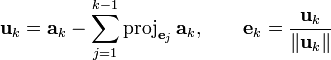
Consider the Gram–Schmidt process, with the vectors to be considered in the process as the columns of the matrix 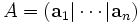 . We define
  where
where  .
.
Then


We then rearrange the equations above so that the  s are on the left, producing the following equations.


Note that since the  are unit vectors, we have the following.


Now the right sides of these equations can be written in matrix form as follows:

But the product of each row and column of the matrices above give us a respective column of A that we started with, and together, they give us the matrix A, so we have factorized A into an orthogonal matrix Q (the matrix of eks), via Gram Schmidt, and the obvious upper triangular matrix as a remainder R.
Alternatively,  can be calculated as follows:
Recall that  Then, we have
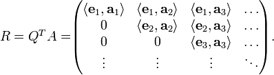
Note that 
 and QQT = I, so QT = Q − 1.
[edit] Example
Consider the decomposition of

Recall that an orthogonal matrix Q has the property

Then, we can calculate Q by means of Gram-Schmidt as follows:


Thus, we have


[edit] Relation to RQ decomposition
The RQ decomposition transforms a matrix A into the product of an upper triangular matrix R (also known as right-triangular) and an orthogonal matrix Q. The only difference from QR decomposition is the order of these matrices.
QR decomposition is Gram-Schmidt orthogonalization of columns of A, started from the first column.
RQ decomposition is Gram-Schmidt orthogonalization of rows of A, started from the last row.
[edit] Using Householder reflections
A Householder reflection (or Householder transformation) is a transformation that takes a vector and reflects it about some plane. We can use this operation to calculate the QR factorization of a matrix.
Q can be used to reflect a vector in such a way that all coordinates but one disappear.
Let  be an arbitrary real m-dimensional column vector such that |||| = |α| for a scalar α. If the algorithm is implemented using floating-point arithmetic, then α should get the opposite sign as the first coordinate of to avoid loss of significance. In the complex case, set

(Stoer & Bulirsch 2002, p. 225) and substitute transposition by conjugate transposition in the construction of Q below.
Then, where  is the vector (1,0,...,0)T, and ||·|| the Euclidean norm, set


If, in case of complex matrix

 is Transpos and conjugate matrix of
Q is a Householder matrix and

This can be used to gradually transform an m-by-n matrix A to upper triangular form. First, we multiply A with the Householder matrix Q1 we obtain when we choose the first matrix column for x. This results in a matrix Q1A with zeros in the left column (except for the first row).

This can be repeated for A′ (obtained from Q1A by deleting the first row and first column), resulting in a Householder matrix Q′2. Note that Q′2 is smaller than Q1. Since we want it really to operate on Q1A instead of A′ we need to expand it to the upper left, filling in a 1, or in general:

After t iterations of this process, t = min(m − 1,n),

is a upper triangular matrix. So, with

A = QR is a QR decomposition of A.
This method has greater numerical stability than the Gram-Schmidt method above.
The following table gives the number of operations in the k-th step of the QR-Decomposition by the Householder transformation, assuming a square matrix with size n.
| Operation | Number of operations in the k-th step |
|---|---|
| multiplications | 2(n − k + 1)2 |
| additions | (n − k + 1)2 + (n − k + 1)(n − k) + 2 |
| division | 1 |
| square root | 1 |
Summing these numbers over the (n − 1) steps (for a square matrix of size n), the complexity of the algorithm (in terms of floating point multiplications) is given by

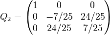
[edit] Example
Let us calculate the decomposition of
First, we need to find a reflection that transforms the first column of matrix A, vector  , to
, to 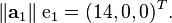
Now,
and

Here,
- α = 14 and

Therefore
 and
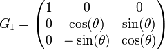
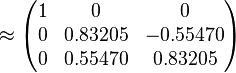
and  , and then


Now observe:

so we already have almost a triangular matrix. We only need to zero the (3, 2) entry.
Take the (1, 1) minor, and then apply the process again to

By the same method as above, we obtain the matrix of the Householder transformation
after performing a direct sum with 1 to make sure the next step in the process works properly.
Now, we find


The matrix Q is orthogonal and R is upper triangular, so A = QR is the required QR-decomposition.
[edit] Using Givens rotations
QR decompositions can also be computed with a series of Givens rotations. Each rotation zeros an element in the subdiagonal of the matrix, forming the R matrix. The concatenation of all the Givens rotations forms the orthogonal Q matrix.
In practice, Givens rotations are not actually performed by building a whole matrix and doing a matrix multiplication. A Givens rotation procedure is used instead which does the equivalent of the sparse Givens matrix multiplication, without the extra work of handling the sparse elements. The Givens rotation procedure is useful in situations where only a relatively few off diagonal elements need to be zeroed, and is more easily parallelized than Householder transformations.
[edit] Example
Let us calculate the decomposition of
First, we need to form a rotation matrix that will zero the lowermost left element,  . We form this matrix using the Givens rotation method, and call the matrix G1. We will first rotate the vector (6, − 4), to point along the X axis. This vector has an angle
  . We create the orthogonal Givens rotation matrix, G1:
And the result of G1A now has a zero in the  element.

We can similarly form Givens matrices G2 and G3, which will zero the sub-diagonal elements a21 and a32, forming a triangular matrix R. The orthogonal matrix QT is formed from the concatenation of all the Givens matrices QT = G3G2G1. Thus, we have G3G2G1A = QTA = R, and the QR decomposition is A = QR.
[edit] Connection to a determinant or a product of eigenvalues
We can use QR decomposition to find the absolute value of the determinant of a square matrix. Suppose a matrix is decomposed as A = QR. Then we have

Since Q is unitary, | det(Q) | = 1. Thus,

where rii are the entries on the diagonal of R.
Furthermore, because the determinant equals the product of the eigenvalues, we have

where λi are eigenvalues of A.
We can extend the above properties to non-square complex matrix A by introducing the definition of QR-decomposition for non-square complex matrix and replacing eigenvalues with singular values.
Suppose a QR decomposition for a non-square matrix A:

where O is a zero matrix and Q is an unitary matrix.
From the properties of SVD and determinant of matrix, we have

where σi are singular values of A.
Note that the singular values of A and R are identical, although the complex eigenvalues of them may be different. However, if A is square, it holds that
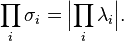
In conclusion, QR decomposition can be used efficiently to calculate a product of eigenvalues or singular values of matrix.
[edit] See also
- Polar decomposition
- Eigenvalue decomposition
- Spectral decomposition
- Matrix decomposition
- Zappa-Szép product
[edit] References
- Golub, Gene H.; Van Loan, Charles F. (1996), Matrix Computations (3rd ed.), Johns Hopkins, ISBN 978-0-8018-5414-9.
- Horn, Roger A.; Johnson, Charles R. (1985), Matrix Analysis, Cambridge University Press, ISBN 0-521-38632-2. Section 2.8.
- Stoer, Josef; Bulirsch, Roland (2002), Introduction to Numerical Analysis (3rd ed.), Springer, ISBN 0-387-95452-X.
- Mezzadri, Francesco (May 2007), "How to Generate Random Matrices from the Classical Compact Groups", Notices (AMS) 54 (5): 592–604, arΧiv:math-ph/0609050, http://www.ams.org/notices/200705/fea-mezzadri-web.pdf.
[edit] External links
- Online Matrix Calculator Performs QR decomposition of matrices.
- LAPACK users manual gives details of subroutines to calculate the QR decomposition
- Mathematica users manual gives details and examples of routines to calculate QR decomposition
- ALGLIB includes a partial port of the LAPACK to C++, C#, Delphi, etc.

