Dipole antenna

From Wikipedia, the free encyclopedia

A schematic of a half-wave dipole antenna that a shortwave listener might build.

Dipole antenna

A dipole antenna, developed by Heinrich Rudolph Hertz around 1886,^{[citation needed]} is an antenna that can be made by a simple wire, with a center-fed driven element for transmitting or receiving radio frequency energy. These antennas are the simplest practical antennas from a theoretical point of view; the current amplitude on such an antenna decreases uniformly from maximum at the center to zero at the ends.

[edit] Elementary doublet

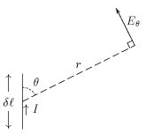
An elementary doublet is a small length of conductor $\scriptstyle{ \delta\ell}$ (small compared with the wavelength $\scriptstyle{\lambda}$ ) traversed by an alternating current:

$\scriptstyle{I=I_\circ e^{i\omega t}}.$

Here $\scriptstyle{\omega=2\pi F}$ is the pulsation (and $\scriptstyle{F}$ the frequency). $\scriptstyle{i}$ is, as usual $\scriptstyle{\sqrt{-1}}$ . This writing using complex numbers is the same as the writing used with phasors or impedances.

Note that this dipole cannot be physically constructed. The circulating current needs somewhere to come from and somewhere to go through. In reality, this small length of conductor will be just one of the multiple segments into which we must divide a real antenna, in order to calculate its proprieties. The interest of this imaginary elementary antenna is that we can easily calculate the far electrical field of the electromagnetic wave radiated by each elementary doublet. We give just the result:

$E_\theta={{-iI_\circ\sin\theta}\over 2\varepsilon_\circ c r}{\delta \ell\over\lambda}e^{i\left(\omega t-kr\right)}$

Where,

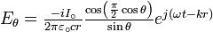
$\scriptstyle{E_\theta}$ is the far electric field of the electromagnetic wave radiated in the $θ$ direction.
$\scriptstyle{\varepsilon_\circ}$ is the permittivity of vacuum.
$\scriptstyle{c}$ is the speed of light in vacuum.
$\scriptstyle{r}$ is the distance from the doublet to the point where the electrical field $\scriptstyle{E_\theta}$ is evaluated.
$\scriptstyle{k}$ is the wavenumber $\scriptstyle{k={2\pi\over\lambda}}$

The exponent of $e\,$ accounts for the phase dependence of the electrical field on time and the distance to the dipole.

The far electric field $\scriptstyle{E_\theta}$ of the electromagnetic wave is coplanar with the conductor and perpendicular with the line joining the dipole to the point where the field is evaluated. If the dipole is placed in the center of a sphere in the axis south-north, the electric field would be parallel to geographic meridians and the magnetic field of the electromagnetic wave would be parallel to geographic parallels.

[edit] Short dipole

A short dipole is a physically feasible dipole formed by two conductors with a total length $\scriptstyle{L}$ very small compared with the wavelength $\scriptstyle{\lambda}$ . The two conducting wires are fed at the centre of the dipole. We assume the hypothesis that the current is maximal at the centre (where the dipole is fed) and that it decreases linearly to be zero at the ends of the wires. Note that the direction of the current is the same in both the dipole branches - to the right in both or to the left in both. The far field $\scriptstyle{E_\theta}$ of the electromagnetic wave radiated by this dipole is:

$E_\theta={-iI_\circ\sin\theta\over 4\varepsilon_\circ c r}{L\over\lambda}e^{i\left(\omega t-kr\right)}.$

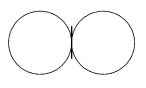
Emission is maximal in the plane perpendicular to the dipole and zero in the direction of wires, that is, the current direction.
The emission diagram is circular section torus shaped (left image) with zero inner diameter. In the right image doublet is vertical in the torus centre.

Knowing this electric field, we can compute the total emitted power and then compute the resistive part of the series impedance of this dipole due to the radiated field, known as the radiation resistance:

$R_{series}={\pi\over6}Z_0 \left({L\over\lambda}\right)^2$ (for $\scriptstyle{L \ll \lambda}$ ).

where $Z 0$ is the impedance of free space. Using a common approximation of $Z 0 = 120π$ ohms, we get:

$R_{series}=20\pi^2\left({L\over\lambda}\right)^2$ ohms

[edit] Antenna gain

Antenna gain is the ratio of surface power radiated by the antenna to the surface power radiated by a hypothetical isotropic antenna:

$G={\left({P\over S}\right)_{ant}\over{\left({P\over S}\right)_{iso}}}$

The surface power carried by an electromagnetic wave is:

$\textstyle{\left({P\over S}\right)_{ant}}=\textstyle{1\over2}c\varepsilon_\circ E_\theta^2\simeq\textstyle{{1\over120\pi}}E_\theta^2$

The surface power radiated by an isotropic antenna feed with the same power is:

$\textstyle{\left({P\over S}\right)_{iso}}=\textstyle{{1\over2} R_{series}I_\circ^2\over4\pi r^2}$

Substituting values for the case of a short dipole, final result is:

$G=\textstyle{{\pi\left({L\over\lambda}\right)^2\over \varepsilon_\circ c{2\pi\over3\varepsilon_\circ c}\left({L\over\lambda}\right)^2}}$ = 1.5 = 1.76 dBi

dBi simply means decibels gain, relative to an isotropic antenna.

[edit] Half-wave antenna

Typically a dipole antenna is formed by two quarter wavelength conductors or elements placed back to back for a total length of $\scriptstyle{\lambda/2}$ . A standing wave on an element of a length ~ $\scriptstyle{\lambda/4}$ yields the greatest voltage differential, as one end of the element is at a node while the other is at an antinode of the wave. The larger the differential voltage, the greater the current flow between the elements.

Assuming a sinusoidal distribution, the current impressed by this voltage differential is given by:

$\textstyle{I=I_\circ e^{i\omega t}\cos{k\ell}}$

For the far-field case, the formula for the electric field of a radiating electromagnetic wave is somewhat more complex:

$\textstyle{E_\theta={-iI_\circ\over 2\pi\varepsilon_\circ c r}}{\cos\left(\scriptstyle{\pi\over 2}\cos\theta\right)\over\sin\theta}e^{j\left(\omega t-kr\right)}$

But the fraction $\textstyle{{\cos\left(\scriptstyle{\pi\over 2}\cos\theta\right)\over\sin\theta}}$ is not very different from $\scriptstyle{\sin\theta}$ .

The resulting emission diagram is a slightly flattened torus.

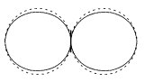
The image on the left shows the section of the emission pattern. We have drawn, in dotted lines, the emission pattern of a short dipole. We can see that the two patterns are very similar. The image at right shows the perspective view of the same emission pattern.

This time it is not possible to compute analytically the total power emitted by the antenna (the last formula does not allow), though a simple numerical integration or series expansion leads to the more precise, actual value of the half-wave resistance:

$\begin{align}R_{\frac{\lambda}{2}} &=60\operatorname{Cin}(2\pi)=60\left[\ln(2\pi\gamma)-\operatorname{Ci}(2\pi)\right]=120\int_{0}^{\frac{\pi}{2}}\frac{\cos\left(\frac{\pi}{2}\cos\theta\right)^2}{\sin\theta}d\theta,\\ &=15\left[2\pi^2-\frac{1}{3}\pi^4+\frac{4}{135}\pi^6-\frac{1}{630}\pi^8+\frac{4}{70875}\pi^{10}\ldots-(-1)^n\frac{(2\pi)^{2n}}{n(2n)!}\right],\\ &=73.12960179171673235432131024310052433236972993\ldots\;\Omega; \end{align}\,\!$

(In most cases 73.1296, or even 73.13, is adequate)

This leads to the gain of a dipole antenna, $G_{\frac{\lambda}{2}}\,\!$ :

$\begin{align}G_{\frac{\lambda}{2}} &=\frac{60^2}{30R_{\frac{\lambda}{2}}}=\frac{3600}{30R_{\frac{\lambda}{2}}}=\frac{120}{R_{\frac{\lambda}{2}}}=\frac{1}{{}^{\int_{0}^{\frac{\pi}{2}}\frac{\cos\left(\frac{\pi}{2}\cos\theta\right)^2}{\sin\theta}d\theta}},\\ &\approx\frac{120}{73.1296}\approx 1.6409224\approx 2.15088\,\mathrm{dBi};\end{align}\,\!$

(Likewise, 1.64 and 2.15 dBi are usually the cited values)

The resistance, however, is not enough to characterize the dipole impedance, as there is also an imaginary part——it is better to measure the impedance.

In the image below, the real and imaginary parts of a dipole's impedance are drawn for lengths going from $\scriptstyle{0.4\,\lambda}\,\!$ to $\scriptstyle{0.6\,\lambda}\,\!$ , accompanied by a chart comparing the gains of dipole antennas of other lengths (note that gains are not in dBi but in natural number):

UHF–Half–Wave Dipole, 1.0–4 GHz

Gain of dipole antennas
length L in $\scriptstyle{\lambda}$	Gain	Gain(dB)
$\scriptstyle{\ll}$ 1	1.50	1.76dB
0.5	1.64	2.15dB
1.0	1.80	2.55dB
1.5	2.00	3.01dB
2.0	2.30	3.62dB
3.0	2.80	4.47dB
4.0	3.50	5.44dB
8.0	7.10	8.51dB

[edit] Quarter-wave antenna

The antenna and its image form a $\scriptstyle{{\lambda\over 2}}$ dipole that radiates only upward.

The quarter wave or unipole antenna is a single element antenna fed at one end, that behaves as a dipole antenna. It is formed by a conductor $\scriptstyle{{\lambda\over 4}}$ in length. It is fed in the lower end, which is near a conductive surface which works as a reflector (see Effect of ground). The current in the reflected image has the same direction and phase that the current in the real antenna. The set quarter-wave plus image forms a half-wave dipole that radiates only in the upper half of space.

In this upper side of space the emitted field has the same amplitude of the field radiated by a half-wave dipole fed with the same current. Therefore, the total emitted power is one-half the emitted power of a half-wave dipole fed with the same current. As the current is the same, the radiation resistance (real part of series impedance) will be one-half of the series impedance of a half-wave dipole. As the reactive part is also divided by 2, the impedance of a quarter wave antenna is $\scriptstyle{{73+i43\over 2}=36+i21}$ ohms. Since the fields above ground are the same as for the dipole, but only half the power is applied, the gain is twice (3dB over) that for a half-wave dipole ( $\scriptstyle{{\lambda\over 2}}$ ), that is 5.14 dBi.

The earth can be used as ground plane. However, the earth is not a good conductor. It is rather a dielectric. The reflected antenna image is good when seen at grazing angles, that is, far from the antenna, but not when seen near the antenna. Far from the antenna and near the ground, electromagnetic fields and radiation patterns are the same as for a half-wave dipole. The impedance is not the same as with a good conductor ground plane. Conductivity of earth surface can be improved with an expensive copper wire mesh.

When ground is not available, as in a vehicle, other metallic surfaces can serve a ground plane, for example the roof of the vehicle. In other situations, radial wires placed at the foot of the quarter-wave wire can simulate a ground plane. For VHF bands, the radiating and groundplane elements can be realised as rigid rods or tubes.

[edit] Dipole characteristics

[edit] Frequency versus length

Dipoles that are much smaller than the wavelength of the signal are called Hertzian, short, or infinitesimal dipoles. These have a very low radiation resistance and a high reactance, making them inefficient, but they are often the only available antennas at very long wavelengths. Dipoles whose length is half the wavelength of the signal are called half-wave dipoles, and are more efficient. In general radio engineering, the term dipole usually means a half-wave dipole (center-fed).

A half-wave dipole is cut to length according to the formula $l\ =\ {468}/{f}$ [ft], where l is the length in feet and f is the center frequency in MHz [1]. This is because the impedance of the dipole is resistive pure at about this length. The metric formula is $l\ =\ {142.65}/{f}$ [m], where l is the length in meters. The length of the dipole antenna is about 95% of half a wavelength at the speed of light in free space.

The magic numbers above are derived from a one Hz wavelength which is the distance that light radio travels in one second. For English that is 186,282 miles times 5280 feet per mile. To convert to metric multiply the previous total by 12 inches per foot and then, by definition, multiply that by 2.54 cm per inch. Divide this number by 100 to convert this length to meters. Then divide the result by one million to account for MHz rather than hertz. This will give a number which must be divided by two for a dipole antenna. To correct for resistance and impedance multiply the dipole wavelength by about 95% to account for the difference in the velocity of wave propagation in wire as opposed to the same wave in free space. If the wire velocity is known, that value should be used to get the magic numbers of 468 feet or 142.65 metric. All that is left is to divide by the desired frequency as measured in MHz to obtain the length of the antenna element.

[edit] Radiation pattern and gain

Dipoles have a toroidal (doughnut-shaped) reception and radiation pattern where the axis of the toroid centers about the dipole. The theoretical maximum gain of a Hertzian dipole is 10 log 1.5 or 1.76 dBi. The maximum theoretical gain of a λ/2-dipole is 10 log 1.64 or 2.15 dBi.

Radiation pattern of a half-wave dipole antenna. The scale is linear.

Gain of a half-wave dipole (same as left). The scale is in dBi (decibels over isotropic).

[edit] Feeder line

Ideally, a half-wave (λ/2) dipole should be fed with a balanced line matching the theoretical 73 ohm impedance of the antenna. A folded dipole uses a 300 ohm balanced feeder line.

Many people have had success in feeding a dipole directly with a coaxial cable feed rather than a ladder-line. However, coax is not symmetrical and thus not a balanced feeder. It is unbalanced, because the outer shield is connected to earth potential at the other end. [2] When a balanced antenna such as a dipole is fed with an unbalanced feeder, common mode currents can cause the coax line to radiate in addition to the antenna itself, and the radiation pattern may be asymmetrically distorted. [3] This can be remedied with the use of a balun.

[edit] Common applications of dipole antennas

[edit] Set-top TV antenna

A "rabbit-ears" antenna with a UHF loop antenna.

The most common dipole antenna is the type used with televisions, often colloquially referred to as "rabbit ears" or "bunny ears." While in most applications the dipole elements are arranged along the same line, rabbit ears are adjustable in length and angle. Larger dipoles are sometimes hung in a V shape with the center near the radio equipment on the ground or the ends on the ground with the center supported. Shorter dipoles can be hung vertically. Some have extra elements to get better reception such as loops (especially for UHF transmissions), which can be turnable around a vertical axis, or a dial, which modifies the electrical properties of the antenna at each dial position.

[edit] Folded dipole

Folded dipole antenna

A DIY-made dipole antenna with mast

Another common place one can see dipoles is as antennas for the FM band - these are folded dipoles. The tips of the antenna are folded back until they almost meet at the feedpoint, such that the antenna comprises one entire wavelength. This arrangement has a greater bandwidth than a standard half-wave dipole. If the conductor has a constant radius and cross-section, at resonance the input impedance is four times that of a half-wave dipole.

[edit] Shortwave antenna

Dipoles for longer wavelengths are made from solid or stranded wire. Portable dipole antennas are made from wire that can be rolled up when not in use. Ropes with weights on the ends can be thrown over supports such as tree branches and then used to hoist up the antenna. The center and the connecting cable can be hoisted up with the ends on the ground or the ends hoisted up between two supports in a V shape. While permanent antennas can be trimmed to the proper length, it is helpful if portable antennas are adjustable to allow for local conditions when moved. One easy way is to fold the ends of the elements to form loops and use adjustable clamps. The loops can then be used as attachment points.

It is important to fit a good insulator at the ends of the dipole, as failure to do so can lead to a flashover if the dipole is used with a transmitter. One cheap insulator is the plastic carrier that holds a pack of beer cans together. This beer can insulator is an example of how a household object can be used in place of an expensive object sold for use as an item of radio equipment. Other objects that can be used as insulators include buttons from old clothing.

[edit] Whip antenna

The whip antenna is probably the most common and simplest-looking antenna. These are monopoles, and the most common and practical is the quarter-wave monopole which could be considered as half of a dipole using a ground plane as the image of the other half. The commonly referred-to end-fed dipole is actually just a half-wave monopole whip antenna.

[edit] Dipoles v whip antennas

Dipoles are generally more efficient than whip antennas (quarter-wave monopoles). The total radiated power and the radiation resistance are twice that of a quarter-wave monopole. Thus, if a whip antenna were used with an infinite perfectly conducting ground plane, then it would be as efficient in half-space as a dipole in free space an infinite distance from any conductive surfaces such as the earth's surface.

[edit] Dipole towers

Large constructed half-wavelength dipole towers include the Warsaw radio mast — the only half-wave dipole for longwave ever built — and Blaw-Knox Towers.

[edit] Military

US Military personnel occasionally use a doublet antenna, especially during dismounted unconventional warfare. A radio operator may choose to bring several doublet antennas for different frequencies, such as an antenna cut to length for the set MEDEVAC (medical evacuation) frequency, NCS (net control station) frequency, and tactical frequency (the frequency used by troops in the field). This approach may not be acceptable depending on the mission. Note that a doublet antenna will not work with the standard SINCGARS radio when using FH (frequency hop) but is effective for SC (single channel). A doublet antenna is more practical for radios not intended for FH.

[edit] Collinear antenna systems based on dipoles

J-Pole Antenna

Dipoles can be stacked end to end in phased arrays to make collinear antenna arrays, which exhibit more gain in certain directions—the toroidal radiation pattern is flattened out, giving maximum gain at right angles to the axis of the colinear array.

[edit] Slim Jim or J-pole

A Slim Jim or J-pole is a form of end-fed dipole connected to a quarter-wave stub matching section.

[edit] Dipole types

[edit] Ideal half-wavelength dipole

This type of antenna is a special case where each wire is exactly one-quarter of the wavelength, for a total of a half wavelength. The radiation resistance is about 73 ohms if wire diameter is ignored, making it easily matched to a coaxial transmission line. The directivity is a constant 1.64, or 2.15 dB. Actual gain will be a little less due to ohmic losses.

If the dipole is not driven at the centre then the feed point resistance will be higher. If the feed point is distance x from one end of a half wave (λ/2) dipole, the resistance will be described by the following equation.

$R_r\ =\ \frac{75}{\sin^2\Big(\frac{2\ \pi\ x}{\lambda}\Big)}$

If taken to the extreme then the feed point resistance of a λ/2 long rod is infinite, but it is possible to use a λ/2 pole as an aerial; the right way to drive it is to connect it to one terminal of a parallel LC resonant circuit. The other side of the circuit must be connected to the braid of a coaxial cable lead and the core of the coaxial cable can be connected part way up the coil from the RF ground side. An alternative means of feeding this system is to use a second coil which is magnetically coupled to the coil attached to the aerial.

[edit] Folded dipole

A folded dipole is a half-wave dipole with an additional wire connecting its two ends. If the additional wire has the same diameter and cross-section as the dipole, two nearly identical radiating currents are generated. The resulting far-field emission pattern is nearly identical to the one for the single-wire dipole described above; however, at resonance its input (feedpoint) impedance $R d f$ is four times the radiation resistance of a single-wire dipole. This is because for a fixed amount of power, the total radiating current $I 0$ is equal to twice the current in each wire and thus equal to twice the current at the feed point. Equating the average radiated power to the average power delivered at the feedpoint, we may write

$\frac{1}{2} R_{\frac{\lambda}{2}} I_0^2 = \frac{1}{2} R_{fd}\left( I_0/2 \right)^2.$

It follows that

$R_{fd}= 4 R_{\frac{\lambda}{2}} = 292.52 \Omega .$

The folded dipole is therefore well matched to 300-Ohm balanced transmission lines.

[edit] Hertzian (i.e. short or infinitesimal) dipole

The Hertzian dipole is a theoretical dipole antenna that consists of an infinitesimally small current source acting in free-space. Although a true Hertzian dipole cannot physically exist, very short dipole antennas can make for a reasonable approximation.

The length of this antenna is significantly smaller than the wavelength:

$l < \frac{\lambda}{50}$

The radiation resistance is given by:

$R_{r} = \frac{2 \pi}{3} Z_{0} \left( \frac{\ell}{\lambda}\right)^{2}.$

where $Z 0$ is the impedance of free space.

The radiation resistance is typically a fraction of an ohm, making the infinitesimal dipole an inefficient radiator. The directivity D, which is the theoretical gain of the antenna assuming no ohmic losses (not real-world), is a constant of 1.5, which corresponds to 1.76 dB. Actual gain will be much less due to the ohmic losses and the loss inherent in connecting a transmission line to the antenna, which is very hard to do efficiently considering the incredibly low radiation resistance. The maximum effective aperture is:

$A_e = \frac{3 \lambda ^2 }{8 \pi}$

A surprising result is that even though the Hertzian dipole is minute, its effective aperture is comparable to antennas many times its size.

[edit] Dipole as a reference standard

Antenna gain is sometimes measured as "x dB above a dipole", which means that the antenna in question is being compared to a dipole, and has x dB more gain (has more directivity) than the dipole tuned to the same operating frequency. In this case one says the antenna has a gain of "x dBd" (see decibel). More often, gains are expressed relative to an isotropic radiator, which is an imaginary aerial that radiates equally in all directions. In this case one uses dBi instead of dBd (see decibel). As it is impossible to build an isotropic radiator, gain measurements expressed relative to a dipole are more practical when a reference dipole aerial is used for experimental measurements. 0 dBd is often considered equal to 2.15 dBi.

A dipole antenna cut from an infinitely large sheet of metal, with sufficient thickness, is complementary to the slot antenna, both giving the same radiation pattern.

[edit] Dipole with baluns

Coax and antenna acting as a radiators instead of only the antenna.

When a dipole is used both to transmit and to receive, the characteristics of the feedline become much more important. Specifically, the antenna must be balanced with the feedline. Failure to do this causes the feedline, in addition to the antenna itself, to radiate. RF can be induced into other electronic equipment near the radiating feedline, causing RF interference. Furthermore, the antenna is not as efficient as it could be because it is radiating closer to the ground and its radiation (and reception) pattern may be distorted asymmetrically. At higher frequencies, where the length of the dipole becomes significantly shorter than the diameter of the feeder coax, this becomes a more significant problem. One solution to this problem is to use a balun.

Several type of baluns are commonly used to transmit on a dipole: current baluns and coax baluns.

[edit] Current balun

Dipole with a current balun.

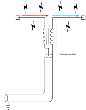
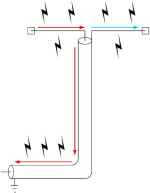
A current balun is a bit more expensive but has the characteristic of being more broadband.[4] It can also be as simple as winding the coax cable over a ferrite core.[5] Or nothing but coax cable:[6]

[edit] Coax balun

Here is a dipole using a coax balun.

A coax balun is a cost effective method to eliminate feeder radiation, but is limited to a narrow set of operating frequencies.

One easy way to make a balun is a (λ/2) length of coaxial cable. The inner core of the cable is linked at each end to one of the balanced connections for a feeder or dipole. One of these terminals should be connected to the inner core of the coaxial feeder. All three braids should be connected together. This then forms a 4:1 balun which works correctly at only a narrow band of frequencies.

[edit] Sleeve balun

Here is a dipole using a sleeve balun.

At VHF frequencies, a sleeve balun can also be built to remove feeder radiation.

Another narrow band design is to use a λ/4 length of metal pipe. The coaxial cable is placed inside the pipe; at one end the braid is wired to the pipe while at the other end no connection is made to the pipe. The balanced end of this balun is at the end where the pipe is wired to the braid. The λ/4 conductor acts as a transformer converting the infinite impedance at the unconnected end into a zero impedance at the end connected to the braid. Hence any current entering the balun through the connection, which goes to the braid at the end with the connection to the pipe, will flow into the pipe. This balun design is not good for low frequencies because of the long length of pipe that will be needed. An easy way to make such a balun is to paint the outside of the coax with conductive paint, then to connect this paint to the braid. Sleeve Baluns

[edit] See also

[edit] References

Elementary, short and half-wave dipoles:

Electronic Radio and Engineering. F.R. Terman. MacGraw-Hill
Lectures on physics. Feynman, Leighton and Sands. Addison-Wesley
Classical Electricity and Magnetism. W. Panofsky and M. Phillips. Addison-Wesley
http://www.ece.rutgers.edu/~orfanidi/ewa/ Electromagnetic Waves and Antennas, Sophocles J. Orfanidis.
Wire Antenna Resources for Ham Radio Wire Antenna Resources including off center fed dipole (OCFD), dipole calculators and construction sites
http://stewks.ece.stevens-tech.edu/sktpersonal.dir/sktwireless/lin-ant.pdf
http://www.nt.hs-bremen.de/peik/asc/asc_antenna_slides.pdf
The Hertzian dipole
ARRL's Wire Antenna Classics - A collection of the best articles from ARRL publications Volume 1. First edition, fifth printing, 2005. © 1999-2005, The American Radio Relay League, Inc. (ISBN 0-87259-707-5)
AC6V's Homebrew Antennas Links
Reflections on Hertz and the Hertzian Dipole Jed Z. Buchwald, MIT and the Dibner Institute for the History of Science and Technology (link inactive February 2, 2007)

[edit] External links

Dipole Antenna Tutorial EM Talk
Broadband Dipoles Antenna-Theory.com

Dipole antenna

From Wikipedia, the free encyclopedia

Contents

[edit] Elementary doublet

[edit] Short dipole

[edit] Antenna gain

[edit] Half-wave antenna

[edit] Quarter-wave antenna

[edit] Dipole characteristics

[edit] Frequency versus length

[edit] Radiation pattern and gain

[edit] Feeder line

[edit] Common applications of dipole antennas

[edit] Set-top TV antenna

[edit] Folded dipole

[edit] Shortwave antenna

[edit] Whip antenna

[edit] Dipoles v whip antennas

[edit] Dipole towers

[edit] Military

[edit] Collinear antenna systems based on dipoles

[edit] Slim Jim or J-pole

[edit] Dipole types

[edit] Ideal half-wavelength dipole

[edit] Folded dipole

[edit] Hertzian (i.e. short or infinitesimal) dipole

[edit] Dipole as a reference standard

[edit] Dipole with baluns

[edit] Current balun

[edit] Coax balun

[edit] Sleeve balun

[edit] See also

[edit] References

[edit] External links

Views

Personal tools

Navigation

Search

Interaction

Toolbox

Languages