Estimation theory

From Wikipedia, the free encyclopedia

Estimation theory is a branch of statistics and signal processing that deals with estimating the values of parameters based on measured/empirical data. The parameters describe an underlying physical setting in such a way that the value of the parameters affects the distribution of the measured data. An estimator attempts to approximate the unknown parameters using the measurements.

For example, it is desired to estimate the proportion of a population of voters who will vote for a particular candidate. That proportion is the unobservable parameter; the estimate is based on a small random sample of voters.

Or, for example, in radar the goal is to estimate the location of objects (airplanes, boats, etc.) by analyzing the received echo and a possible question to be posed is "where are the airplanes?" To answer where the airplanes are, it is necessary to estimate the distance the airplanes are at from the radar station, which can provide an absolute location if the absolute location of the radar station is known.

In estimation theory, it is assumed that the desired information is embedded in a noisy signal. Noise adds uncertainty, without which the problem would be deterministic and estimation would not be needed.

[edit] Estimation process

The entire purpose of estimation theory is to arrive at an estimator, and preferably an implementable one that could actually be used. The estimator takes the measured data as input and produces an estimate of the parameters.

It is also preferable to derive an estimator that exhibits optimality. An optimal estimator would indicate that all available information in the measured data has been extracted, for if there was unused information in the data then the estimator would not be optimal.

These are the general steps to arrive at an estimator:

In order to arrive at a desired estimator for estimating a single or multiple parameters, it is first necessary to determine a model for the system. This model should incorporate the process being modeled as well as points of uncertainty and noise. The model describes the physical scenario in which the parameters apply.
After deciding upon a model, it is helpful to find the limitations placed upon an estimator. This limitation, for example, can be found through the Cramér-Rao bound.
Next, an estimator needs to be developed or applied if an already known estimator is valid for the model. The estimator needs to be tested against the limitations to determine if it is an optimal estimator (if so, then no other estimator will perform better).
Finally, experiments or simulations can be run using the estimator to test its performance.

After arriving at an estimator, real data might show that the model used to derive the estimator is incorrect, which may require repeating these steps to find a new estimator. A non-implementable or infeasible estimator may need to be scrapped and the process started anew.

In summary, the estimator estimates the parameters of a physical model based on measured data.

[edit] Basics

To build a model, several statistical "ingredients" need to be known. These are needed to ensure the estimator has some mathematical tractability instead of being based on "good feel".

The first is a set of statistical samples taken from a random vector (RV) of size N. Put into a vector,

$\mathbf{x} = \begin{bmatrix} x[0] \\ x[1] \\ \vdots \\ x[N-1] \end{bmatrix}.$

Secondly, we have the corresponding M parameters

$\mathbf{\theta} = \begin{bmatrix} \theta_1 \\ \theta_2 \\ \vdots \\ \theta_M \end{bmatrix},$

which need to be established with their probability density function (pdf) or probability mass function (pmf)

$p(\mathbf{x} | \mathbf{\theta}).\,$

It is also possible for the parameters themselves to have a probability distribution (e.g., Bayesian statistics). It is then necessary to define the epistemic probability

$\pi( \mathbf{\theta}).\,$

After the model is formed, the goal is to estimate the parameters, commonly denoted $\hat{\mathbf{\theta}}$ , where the "hat" indicates the estimate.

One common estimator is the minimum mean squared error (MMSE) estimator, which utilizes the error between the estimated parameters and the actual value of the parameters

$\mathbf{e} = \hat{\mathbf{\theta}} - \mathbf{\theta}$

as the basis for optimality. This error term is then squared and minimized for the MMSE estimator.

[edit] Estimators

Commonly-used estimators and estimation methods, and topics related to them:

Maximum likelihood estimators
Bayes estimators
Method of moments estimators
Cramér-Rao bound
Minimum mean squared error (MMSE), also known as Bayes least squared error (BLSE)
Maximum a posteriori (MAP)
Minimum variance unbiased estimator (MVUE)
Best linear unbiased estimator (BLUE)
Unbiased estimators — see estimator bias.
Particle filter
Markov chain Monte Carlo (MCMC)
Kalman filter
Ensemble Kalman filter (EnKF)
Wiener filter

[edit] Examples

[edit] Unknown constant in additive white Gaussian noise

Consider a received discrete signal, $x [n]$ , of $N$ independent samples that consists of an unknown constant $A$ with additive white Gaussian noise $w [n]$ with known variance $σ 2$ (i.e., $\mathcal{N}(0, \sigma^2)$ ). Since the variance is known then the only unknown parameter is $A$ .

The model for the signal is then

$x[n] = A + w[n] \quad n=0, 1, \dots, N-1$

Two possible (of many) estimators are:

$\hat{A}_1 = x[0]$
$\hat{A}_2 = \frac{1}{N} \sum_{n=0}^{N-1} x[n]$ which is the sample mean

Both of these estimators have a mean of $A$ , which can be shown through taking the expected value of each estimator

$\mathrm{E}\left[\hat{A}_1\right] = \mathrm{E}\left[ x[0] \right] = A$

and

$\mathrm{E}\left[ \hat{A}_2 \right] = \mathrm{E}\left[ \frac{1}{N} \sum_{n=0}^{N-1} x[n] \right] = \frac{1}{N} \left[ \sum_{n=0}^{N-1} \mathrm{E}\left[ x[n] \right] \right] = \frac{1}{N} \left[ N A \right] = A$

At this point, these two estimators would appear to perform the same. However, the difference between them becomes apparent when comparing the variances.

$\mathrm{var} \left( \hat{A}_1 \right) = \mathrm{var} \left( x[0] \right) = \sigma^2$

and

$\mathrm{var} \left( \hat{A}_2 \right) = \mathrm{var} \left( \frac{1}{N} \sum_{n=0}^{N-1} x[n] \right) \overset{independence}{=} \frac{1}{N^2} \left[ \sum_{n=0}^{N-1} \mathrm{var} (x[n]) \right] = \frac{1}{N^2} \left[ N \sigma^2 \right] = \frac{\sigma^2}{N}$

It would seem that the sample mean is a better estimator since, as $N \to \infty$ , the variance goes to zero.

[edit] Maximum likelihood

Main article: Maximum likelihood

Continuing the example using the maximum likelihood estimator, the probability density function (pdf) of the noise for one sample $w [n]$ is

$p(w[n]) = \frac{1}{\sigma \sqrt{2 \pi}} \exp\left(- \frac{1}{2 \sigma^2} w[n]^2 \right)$

and the probability of $x [n]$ becomes ( $x [n]$ can be thought of a $\mathcal{N}(A, \sigma^2)$ )

$p(x[n]; A) = \frac{1}{\sigma \sqrt{2 \pi}} \exp\left(- \frac{1}{2 \sigma^2} (x[n] - A)^2 \right)$

By independence, the probability of $\mathbf{x}$ becomes

$p(\mathbf{x}; A) = \prod_{n=0}^{N-1} p(x[n]; A) = \frac{1}{\left(\sigma \sqrt{2\pi}\right)^N} \exp\left(- \frac{1}{2 \sigma^2} \sum_{n=0}^{N-1}(x[n] - A)^2 \right)$

Taking the natural logarithm of the pdf

$\ln p(\mathbf{x}; A) = -N \ln \left(\sigma \sqrt{2\pi}\right) - \frac{1}{2 \sigma^2} \sum_{n=0}^{N-1}(x[n] - A)^2$

and the maximum likelihood estimator is

$\hat{A} = \arg \max \ln p(\mathbf{x}; A)$

Taking the first derivative of the log-likelihood function

$\frac{\partial}{\partial A} \ln p(\mathbf{x}; A) = \frac{1}{\sigma^2} \left[ \sum_{n=0}^{N-1}(x[n] - A) \right] = \frac{1}{\sigma^2} \left[ \sum_{n=0}^{N-1}x[n] - N A \right]$

and setting it to zero

$0 = \frac{1}{\sigma^2} \left[ \sum_{n=0}^{N-1}x[n] - N A \right] = \sum_{n=0}^{N-1}x[n] - N A$

This results in the maximum likelihood estimator

$\hat{A} = \frac{1}{N} \sum_{n=0}^{N-1}x[n]$

which is simply the sample mean. From this example, it was found that the sample mean is the maximum likelihood estimator for $N$ samples of a fixed, unknown parameter corrupted by AWGN.

[edit] Cramér–Rao lower bound

For more details on this topic, see Cramér–Rao bound.

To find the Cramér-Rao lower bound (CRLB) of the sample mean estimator, it is first necessary to find the Fisher information number

$\mathcal{I}(A) = \mathrm{E} \left( \left[ \frac{\partial}{\partial\theta} \ln p(\mathbf{x}; A) \right]^2 \right) = -\mathrm{E} \left[ \frac{\partial^2}{\partial\theta^2} \ln p(\mathbf{x}; A) \right]$

and copying from above

$\frac{\partial}{\partial A} \ln p(\mathbf{x}; A) = \frac{1}{\sigma^2} \left[ \sum_{n=0}^{N-1}x[n] - N A \right]$

Taking the second derivative

$\frac{\partial^2}{\partial A^2} \ln p(\mathbf{x}; A) = \frac{1}{\sigma^2} (- N) = \frac{-N}{\sigma^2}$

and finding the negative expected value is trivial since it is now a deterministic constant $-\mathrm{E} \left[ \frac{\partial^2}{\partial A^2} \ln p(\mathbf{x}; A) \right] = \frac{N}{\sigma^2}$

Finally, putting the Fisher information into

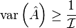
$\mathrm{var}\left( \hat{A} \right) \geq \frac{1}{\mathcal{I}}$

results in

$\mathrm{var}\left( \hat{A} \right) \geq \frac{\sigma^2}{N}$

Comparing this to the variance of the sample mean (determined previously) shows that the sample mean is equal to the Cramér-Rao lower bound for all values of $N$ and $A$ . In other words, the sample mean is the (necessarily unique) efficient estimator, and thus also the minimum variance unbiased estimator (MVUE), in addition to being the maximum likelihood estimator.

[edit] Maximum of a uniform distribution

Main article: German tank problem

One of the simplest non-trivial examples of estimation is the estimation of the maximum of a uniform distribution. It is used as a hands-on classroom exercise and to illustrate basic principles of estimation theory. Further, in the case of estimation based on a single sample, it demonstrates philosophical issues and possible misunderstandings in the use of maximum likelihood estimators and likelihood functions.

Given a discrete uniform distribution $1,2,\dots,N$ with unknown maximum, the UMVU estimator for the maximum is given by

$\frac{k+1}{k} m - 1 = m + \frac{m}{k} - 1$

where m is the sample maximum and k is the sample size, sampling without replacement.^[1]^[2] This problem is commonly known as the German tank problem, due to application of maximum estimation to estimates of German tank production during World War II.

The formula may be understood intuitively as:

"The sample maximum plus the average gap between observations in the sample",

the gap being added to compensate for the negative bias of the sample maximum as an estimator for the population maximum.^{[note 1]}

This has a variance of^[1]

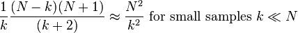
$\frac{1}{k}\frac{(N-k)(N+1)}{(k+2)} \approx \frac{N^2}{k^2} \text{ for small samples } k \ll N$

so a standard deviation of approximately $N / k$ , the (population) average size of a gap between samples; compare $\frac{m}{k}$ above. This can be seen as a very simple case of maximum spacing estimation.

The sample maximum is the maximum likelihood estimator for the population maximum, but, as discussed above, it is biased.

[edit] Applications

Numerous fields require the use of estimation theory. Some of these fields include (but are by no means limited to):

Interpretation of scientific experiments
Signal processing
Clinical trials
Opinion polls
Quality control
Telecommunications
Project management
Software engineering
Control theory
Network intrusion detection system
Orbit Determination

Measured data are likely to be subject to noise or uncertainty and it is through statistical probability that optimal solutions are sought to extract as much information from the data as possible.

[edit] See also

[edit] Notes

^ The sample maximum is never more than the population maximum, but can be less, hence it is a biased estimator: it will tend to underestimate the population maximum.

[edit] References

^ ^a ^b Johnson, Roger (1994), "Estimating the Size of a Population", Teaching Statistics 16 (2 (Summer)), doi:10.1111/j.1467-9639.1994.tb00688.x
^ Johnson, Roger (2006), "Estimating the Size of a Population", Getting the Best from Teaching Statistics, http://www.rsscse.org.uk/ts/gtb/johnson.pdf

[edit] Reference list

Mathematical Statistics and Data Analysis by John Rice. (ISBN 0-534-209343)
Fundamentals of Statistical Signal Processing: Estimation Theory by Steven M. Kay (ISBN 0-13-345711-7)
An Introduction to Signal Detection and Estimation by H. Vincent Poor (ISBN 0-387-94173-8)
Detection, Estimation, and Modulation Theory, Part 1 by Harry L. Van Trees (ISBN 0-471-09517-6; website)
Optimal State Estimation: Kalman, H-infinity, and Nonlinear Approaches by Dan Simon website

[2] The sample maximum is never more than the population maximum, but can be less, hence it is a biased estimator: it will tend to underestimate the population maximum.

[Johnson-0] Johnson, Roger (1994), "Estimating the Size of a Population", Teaching Statistics 16 (2 (Summer)), doi:10.1111/j.1467-9639.1994.tb00688.x

[Johnson2-1] Johnson, Roger (2006), "Estimating the Size of a Population", Getting the Best from Teaching Statistics, http://www.rsscse.org.uk/ts/gtb/johnson.pdf

[1]

[2]

[note 1]

Estimation theory

From Wikipedia, the free encyclopedia

Contents

[edit] Estimation process

[edit] Basics

[edit] Estimators

[edit] Examples

[edit] Unknown constant in additive white Gaussian noise

[edit] Maximum likelihood

[edit] Cramér–Rao lower bound

[edit] Maximum of a uniform distribution

[edit] Applications

[edit] See also

[edit] Notes

[edit] References

[edit] Reference list

Views

Personal tools

Navigation

Search

Interaction

Toolbox

Languages