Autoregressive moving average model
From Wikipedia, the free encyclopedia
In statistics and signal processing, autoregressive moving average (ARMA) models, sometimes called Box-Jenkins models after the iterative Box-Jenkins methodology usually used to estimate them, are typically applied to time series data.
Given a time series of data Xt, the ARMA model is a tool for understanding and, perhaps, predicting future values in this series. The model consists of two parts, an autoregressive (AR) part and a moving average (MA) part. The model is usually then referred to as the ARMA(p,q) model where p is the order of the autoregressive part and q is the order of the moving average part (as defined below).
Contents |
[edit] Autoregressive model
The notation AR(p) refers to the autoregressive model of order p. The AR(p) model is written
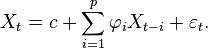
where  are the parameters of the model, c is a constant and
  is white noise. The constant term is omitted by many authors for simplicity.
An autoregressive model is essentially an all-pole infinite impulse response filter with some additional interpretation placed on it.
Some constraints are necessary on the values of the parameters of this model in order that the model remains stationary. For example, processes in the AR(1) model with |φ1| ≥ 1 are not stationary.
[edit] Moving average model
The notation MA(q) refers to the moving average model of order q:

where the θ1, ..., θq are the parameters of the model and the ,  ,... are again, the error terms. The moving average model is essentially a finite impulse response filter with some additional interpretation placed on it.
[edit] Autoregressive moving average model
The notation ARMA(p, q) refers to the model with p autoregressive terms and q moving average terms. This model contains the AR(p) and MA(q) models,

[edit] Note about the error terms
The error terms are generally assumed to be independent identically-distributed random variables (i.i.d.) sampled from a normal distribution with zero mean: ~ N(0,σ2) where σ2 is the variance. These assumptions may be weakened but doing so will change the properties of the model. In particular, a change to the i.i.d. assumption would make a rather fundamental difference.
[edit] Specification in terms of lag operator
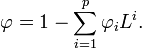
In some texts the models will be specified in terms of the lag operator L. In these terms then the AR(p) model is given by

where φ represents the polynomial
The MA(q) model is given by

where θ represents the polynomial

Finally, the combined ARMA(p, q) model is given by

or more concisely,

[edit] Alternative notation
Some authors, including Box, Jenkins & Reinsel (1994) use a different convention for the autoregression coefficients. This allows all the polynomials involving the lag operator to appear in a similar form throughout. Thus the ARMA model would be written as

[edit] Fitting models
ARMA models in general can, after choosing p and q, be fitted by least squares regression to find the values of the parameters which minimize the error term. It is generally considered good practice to find the smallest values of p and q which provide an acceptable fit to the data. For a pure AR model the Yule-Walker equations may be used to provide a fit.
[edit] Implementations in statistics packages
- In R, the tseries package includes an arma function. The function is documented in "Fit ARMA Models to Time Series".
- MATLAB includes a function ar to estimate AR models, see here for more details.
- gretl can also estimate ARMA models, see here where it's mentioned.
[edit] Applications
ARMA is appropriate when a system is a function of a series of unobserved shocks (the MA part)[clarification needed] as well as its own behavior. For example, stock prices may be shocked by fundamental information as well as exhibiting technical trending and mean-reversion effects due to market participants.
[edit] Generalizations
The dependence of Xt on past values and the error terms εt is assumed to be linear unless specified otherwise. If the dependence is nonlinear, the model is specifically called a nonlinear moving average (NMA), nonlinear autoregressive (NAR), or nonlinear autoregressive moving average (NARMA) model.
Autoregressive moving average models can be generalized in other ways. See also autoregressive conditional heteroskedasticity (ARCH) models and autoregressive integrated moving average (ARIMA) models. If multiple time series are to be fitted then a vector ARIMA (or VARIMA) model may be fitted. If the time-series in question exhibits long memory then fractional ARIMA (FARIMA, sometimes called ARFIMA) modelling may be appropriate: see Autoregressive fractionally integrated moving average. If the data is thought to contain seasonal effects, it may be modeled by a SARIMA (seasonal ARIMA) or a periodic ARMA model.
Another generalization is the multiscale autoregressive (MAR) model. A MAR model is indexed by the nodes of a tree, whereas a standard (discrete time) autoregressive model is indexed by integers. See multiscale autoregressive model for a list of references.
Note that the ARMA model is an univariate model. Extensions for the multivariate case are the Vector Autoregression (VAR) and Vector Autoregression Moving-Average (VARMA).
[edit] Autoregressive moving average model with exogenous inputs model (ARMAX model)
The notation ARMAX(p, q, b) refers to the model with p autoregressive terms, q moving average terms and b eXogenous inputs terms. This model contains the AR(p) and MA(q) models and a linear combination of the last b terms of a known and external time series dt. It is given by:

where  are the parameters of the exogenous input dt.
Some nonlinear variants of models with exogenous variables have been defined: see for example Nonlinear autoregressive exogenous model.
[edit] See also
[edit] References
- George Box, Gwilym M. Jenkins, and Gregory C. Reinsel. Time Series Analysis: Forecasting and Control, third edition. Prentice-Hall, 1994.
- Mills, Terence C. Time Series Techniques for Economists. Cambridge University Press, 1990.
- Percival, Donald B. and Andrew T. Walden. Spectral Analysis for Physical Applications. Cambridge University Press, 1993.
- Pandit, Sudhakar M. and Wu, Shien-Ming. Time Series and System Analysis with Applications. John Wiley & Sons, Inc., 1983.

