Cross-correlation

From Wikipedia, the free encyclopedia

In signal processing, cross-correlation is a measure of similarity of two waveforms as a function of a time-lag applied to one of them. This is also known as a sliding dot product or inner-product. It is commonly used to search a long duration signal for a shorter, known feature. It also has applications in pattern recognition, single particle analysis, electron tomographic averaging, and cryptanalysis.

For continuous functions, f and g, the cross-correlation is defined as:

$(f \star g)(t)\ \stackrel{\mathrm{def}}{=} \int_{-\infty}^{\infty} f^*(\tau)\ g(t+\tau)\,d\tau,$

where f * denotes the complex conjugate of f.

Similarly, for discrete functions, the cross-correlation is defined as:

$(f \star g)[n]\ \stackrel{\mathrm{def}}{=} \sum_{m=-\infty}^{\infty} f^*[m]\ g[n+m].$

The cross-correlation is similar in nature to the convolution of two functions. Whereas convolution involves reversing a signal, then shifting it and multiplying by another signal, correlation only involves shifting it and multiplying (no reversing).

In an Autocorrelation, which is the cross-correlation of a signal with itself, there will always be a peak at a lag of zero.

If $X$ and $Y$ are two independent random variables with probability distributions f and g, respectively, then the probability distribution of the difference $X - Y$ is given by the cross-correlation f $\star$ g. In contrast, the convolution f $*$ g gives the probability distribution of the sum $X + Y$ .

In probability theory and statistics, the term cross-correlation is also sometimes used to refer to the covariance cov(X, Y) between two random vectors X and Y, in order to distinguish that concept from the "covariance" of a random vector X, which is understood to be the matrix of covariances between the scalar components of X.

[edit] Explanation

For example, consider two real valued functions $f$ and $g$ that differ only by a shift along the x-axis. One can calculate the cross-correlation to figure out how much $g$ must be shifted along the x-axis to make it identical to $f$ . The formula essentially slides the $g$ function along the x-axis, calculating the integral of their product for each possible amount of sliding. When the functions match, the value of $(f\star g)$ is maximized. The reason for this is that when lumps (positives areas) are aligned, they contribute to making the integral larger. Also, when the troughs (negative areas) align, they also make a positive contribution to the integral because the product of two negative numbers is positive.

With complex-valued functions $f$ and $g$ , taking the conjugate of $f$ ensures that aligned lumps (or aligned troughs) with imaginary components will contribute positively to the integral.

In econometrics, lagged cross-correlation is sometimes referred to as cross-autocorrelation^[1]

[edit] Properties

The cross-correlation of functions f(t) and g(t) is equivalent to the convolution of f *(−t) and g(t). I.e.:

$f\star g = (t \mapsto f^*(-t))*g.$

If either f or g is Hermitian, then: $f\star g = f*g.$

$(f\star g)\star(f\star g)=(f\star f)\star (g\star g)$

Analogous to the convolution theorem, the cross-correlation satisfies:

$\mathcal{F}\{f\star g\}=(\mathcal{F}\{f\})^* \cdot \mathcal{F}\{g\},$

where $\mathcal{F}$ denotes the Fourier transform, and an asterisk again indicates the complex conjugate. Coupled with fast Fourier transform algorithms, this property is often exploited for the efficient numerical computation of cross-correlations. (see circular cross-correlation)

The cross-correlation is related to the spectral density. (see Wiener–Khinchin theorem)

The cross correlation of a convolution of f and h with a function g is the convolution of the correlation of f and g with the kernel h:

$(f * h) \star g = h(-)*(f \star g)$

[edit] Normalized cross-correlation

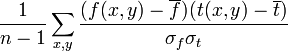
For image-processing applications in which the brightness of the image and template can vary due to lighting and exposure conditions, the images can be first normalized. This is typically done at every step by subtracting the mean and dividing by the standard deviation. That is, the cross-correlation of a template, $t (x, y)$ with a subimage $f (x, y)$ is

$\frac{1}{n-1} \sum_{x,y}\frac{(f(x,y) - \overline{f})(t(x,y) - \overline{t})}{\sigma_f \sigma_t}$ .

where $n$ is the number of pixels in $t (x, y)$ and $f (x, y)$ . In functional analysis terms, this can be thought of as the dot product of two normalized vectors. That is, if