Mandelbrot set

From Wikipedia, the free encyclopedia

Initial image of a Mandelbrot set zoom sequence with continuously coloured environment

In mathematics, the Mandelbrot set, named after Benoît Mandelbrot, is a set of points in the complex plane, the boundary of which forms a fractal. Mathematically, the Mandelbrot set can be defined as the set of complex values of c for which the orbit of 0 under iteration of the complex quadratic polynomial z_n+1 = z_n² + c remains bounded.^[1] That is, a complex number, c, is in the Mandelbrot set if, when starting with z₀=0 and applying the iteration repeatedly, the absolute value of z_n never exceeds a certain number (that number depends on c) however large n gets.

For example, letting c = 1 gives the sequence 0, 1, 2, 5, 26,…, which tends to infinity. As this sequence is unbounded, 1 is not an element of the Mandelbrot set.

On the other hand, c = i gives the sequence 0, i, (−1 + i), −i, (−1 + i), −i…, which is bounded, and so i belongs to the Mandelbrot set.

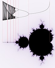
When computed and graphed on the complex plane, the Mandelbrot Set is seen to have an elaborate boundary, which does not simplify at any given magnification. This qualifies the boundary as a fractal.

The Mandelbrot set has become popular outside mathematics both for its aesthetic appeal and for being a complicated structure arising from a simple definition. Benoît Mandelbrot and others worked hard to communicate this area of mathematics to the public.

[edit] History

The Mandelbrot set has its place in complex dynamics, a field first investigated by the French mathematicians Pierre Fatou and Gaston Julia at the beginning of the 20th century. The first pictures of it were drawn in 1978 by Robert Brooks and Peter Matelski as part of a study of Kleinian Groups.^[2]

Mandelbrot studied the parameter space of quadratic polynomials in an article that appeared in 1980.^[3] The mathematical study of the Mandelbrot set really began with work by the mathematicians Adrien Douady and John H. Hubbard,^[4] who established many of its fundamental properties and named the set in honour of Mandelbrot.

The mathematicians Heinz-Otto Peitgen and Peter Richter became well-known for promoting the set with stunning photographs, books,^[5] and an internationally touring exhibit of the German Goethe-Institut.^[6]^[7]

The cover article of the August 1985 Scientific American introduced the algorithm for computing the Mandelbrot set to a wide audience. The cover featured an image created by Peitgen, et. al.^[8]^[9]

The work of Douady and Hubbard coincided with a huge increase in interest in complex dynamics and abstract mathematics, and the study of the Mandelbrot set has been a centerpiece of this field ever since. An exhaustive list of all the mathematicians who have contributed to the understanding of this set since then is beyond the scope of this article, but such a list would notably include Mikhail Lyubich,^[10]^[11] Curt McMullen, John Milnor, Mitsuhiro Shishikura, and Jean-Christophe Yoccoz.

[edit] Formal definition

The Mandelbrot set $M$ is defined by a family of complex quadratic polynomials

$P_c:\mathbb C\to\mathbb C$

given by

$P_c: z\to z^2 + c$ ,

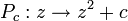where $c$ is a complex parameter. For each $c$ , one considers the behavior of the sequence $(0, P_c(0), P_c(P_c(0)), P_c(P_c(P_c(0))), \ldots)$ obtained by iterating $P c (z)$ starting at critical point $z = 0$ , which either escapes to infinity or stays within a disk of some finite radius. The Mandelbrot set is defined as the set of all points $c$ such that the above sequence does not escape to infinity.

A mathematician's depiction of the Mandelbrot set M, a point c is coloured black if it belongs to the set, and white if not. Re[c] and Im[c] denote the real and imaginary parts of c.

More formally, if $P_c^{\circ n}(z)$ denotes the nth iterate of $P c (z)$ (i.e. $P c (z)$ composed with itself n times), the Mandelbrot set is the subset of the complex plane given by

$M = \left\{c\in \mathbb C : \sup_{n\in \mathbb N}|P_c^{\circ n}(0)| < \infin\right\}.$

Mathematically, the Mandelbrot set is just a set of complex numbers. A given complex number c either belongs to M or it does not. A picture of the Mandelbrot set can be made by colouring all the points $c$ which belong to M black, and all other points white. The more colourful pictures usually seen are generated by colouring points not in the set according to how quickly or slowly the sequence $|P_c^{\circ n}(0)|$ diverges to infinity. See the section on computer drawings below for more details.

The Mandelbrot set can also be defined as the connectedness locus of the family of polynomials $P c (z)$ . That is, it is the subset of the complex plane consisting of those parameters $c$ for which the Julia set of $P c$ is connected.

[edit] Basic properties

The Mandelbrot set is a compact set, contained in the closed disk of radius 2 around the origin. In fact, a point $c$ belongs to the Mandelbrot set if and only if $|P_c^{\circ n}(0)|\leq 2$ for all $n\geq 0$ . In other words, if the absolute value of $P_c^{\circ n}(0)$ ever becomes larger than 2, the sequence will escape to infinity.

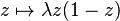
Correspondence between the mandelbrot set and the logistic map

The intersection of $M$ with the real axis is precisely the interval $[-2 , 0.25]\,$ . The parameters along this interval can be put in one-to-one correspondence with those of the real logistic family,

$z\mapsto \lambda z(1-z),\quad \lambda\in[1,4].\,$

The correspondence is given by

$c = \frac{1-(\lambda-1)^2}{4}.$

In fact, this gives a correspondence between the entire parameter space of the logistic family and that of the Mandelbrot set.

The area of the Mandelbrot set is estimated to be 1.506 591 77 ± 0.000 000 08.^[12]

Douady and Hubbard have shown that the Mandelbrot set is connected. In fact, they constructed an explicit conformal isomorphism between the complement of the Mandelbrot set and the complement of the closed unit disk. Mandelbrot had originally conjectured that the Mandelbrot set is disconnected. This conjecture was based on computer pictures generated by programs which are unable to detect the thin filaments connecting different parts of $M$ . Upon further experiments, he revised his conjecture, deciding that $M$ should be connected.

The dynamical formula for the uniformisation of the complement of the Mandelbrot set, arising from Douady and Hubbard's proof of the connectedness of $M$ , gives rise to external rays of the Mandelbrot set. These rays can be used to study the Mandelbrot set in combinatorial terms and form the backbone of the Yoccoz parapuzzle.

The boundary of the Mandelbrot set is exactly the bifurcation locus of the quadratic family; that is, the set of parameters $c$ for which the dynamics changes abruptly under small changes of $c .$ It can be constructed as the limit set of a sequence of plane algebraic curves, the Mandelbrot curves, of the general type known as polynomial lemniscates. The Mandelbrot curves are defined by setting p₀=z, p_n=p_n-1²+z, and then interpreting the set of points |p_n(z)|=1 in the complex plane as a curve in the real Cartesian plane of degree 2ⁿ⁺¹ in x and y.

[edit] Other properties

[edit] The main cardioid and period bulbs

Periods of hyperbolic components

Upon looking at a picture of the Mandelbrot set, one immediately notices the large cardioid-shaped region in the center. This main cardioid is the region of parameters $c$ for which $P c$ has an attracting fixed point. It consists of all parameters of the form

$c = \frac{1-(\mu-1)^2}{4}$

for some $μ$ in the open unit disk.

To the left of the main cardioid, attached to it at the point $c = - 3 / 4$ , a circular-shaped bulb is visible. This bulb consists of those parameters $c$ for which $P c$ has an attracting cycle of period 2. This set of parameters is an actual circle, namely that of radius 1/4 around -1.

There are infinitely many other bulbs tangent to the main cardioid: for every rational number $\textstyle\frac{p}{q}$ , with p and q coprime, there is such a bulb that is tangent at the parameter

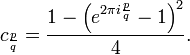
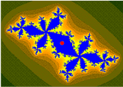
$c_{\frac{p}{q}} = \frac{1 - \left(e^{2\pi i \frac{p}{q}}-1\right)^2}{4}.$

Attracting cycle in 2/5-bulb plotted over Julia set (animation)

This bulb is called the $\textstyle\frac{p}{q}$ -bulb of the Mandelbrot set. It consists of parameters which have an attracting cycle of period $q$ and combinatorial rotation number $\textstyle\frac{p}{q}$ . More precisely, the $q$ periodic Fatou components containing the attracting cycle all touch at a common point (commonly called the $α$ -fixed point). If we label these components $U_0,\dots,U_{q-1}$ in counterclockwise orientation, then $P c$ maps the component $U j$ to the component $U_{j+p\,(\operatorname{mod} q)}$ .

Attracting cycles and Julia sets for parameters in the 1/2, 3/7, 2/5, 1/3, 1/4, and 1/5 bulbs

cycle periods and antennae

The change of behavior occurring at $c_{\frac{p}{q}}$ is known as a bifurcation: the attracting fixed point "collides" with a repelling period q-cycle. As we pass through the bifurcation parameter into the $\textstyle\frac{p}{q}$ -bulb, the attracting fixed point turns into a repelling fixed point (the $α$ -fixed point), and the period q-cycle becomes attracting.

[edit] Hyperbolic components

All the bulbs we encountered in the previous section were interior components of the Mandelbrot set in which the maps $P c$ have an attracting periodic cycle. Such components are called hyperbolic components.

It is conjectured that these are the only interior regions of $M$ . This problem, known as density of hyperbolicity, may be the most important open problem in the field of complex dynamics. Hypothetical non-hyperbolic components of the Mandelbrot set are often referred to as "queer" components.

For real quadratic polynomials, this question was answered positively in the 1990s independently by Lyubich and by Graczyk and Świątek. (Note that hyperbolic components intersecting the real axis correspond exactly to periodic windows in the Feigenbaum diagram. So this result states that such windows exist near every parameter in the diagram.)

Not every hyperbolic component can be reached by a sequence of direct bifurcations from the main cardioid of the Mandelbrot set. However, such a component can be reached by a sequence of direct bifurcations from the main cardioid of a little Mandelbrot copy (see below).

[edit] Local connectivity

It is conjectured that the Mandelbrot set is locally connected. This famous conjecture is known as MLC (for Mandelbrot Locally Connected). By the work of Adrien Douady and John H. Hubbard, this conjecture would result in a simple abstract "pinched disk" model of the Mandelbrot set. In particular, it would imply the important hyperbolicity conjecture mentioned above.

The celebrated work of Jean-Christophe Yoccoz^{[citation needed]}established local connectivity of the Mandelbrot set at all finitely-renormalizable parameters; that is, roughly speaking those which are contained only in finitely many small Mandelbrot copies. Since then, local connectivity has been proved at many other points of $M$ , but the full conjecture is still open.

[edit] Self-similarity

Self similarity in the Mandelbrot set shown by zooming in on a round feature while panning in the negative-x direction. The display center pans from (−1, 0) to (−1.31, 0) while the view magnifies from 0.5 × 0.5 to 0.12 × 0.12 to approximate the Feigenbaum ratio

δ

.

Self-similarity around Misiurewicz point −0.1011 + 0.9563i.

The Mandelbrot set is self-similar under magnification in the neighborhoods of the Misiurewicz points. It is also conjectured to be self-similar around generalized Feigenbaum points (e.g. −1.401155 or −0.1528 + 1.0397i), in the sense of converging to a limit set.^[13]^[14]

Quasi-self-similarity in the Mandelbrot set

The Mandelbrot set in general is not strictly self-similar but it is quasi-self-similar, as small slightly different versions of itself can be found at arbitrarily small scales.

The little copies of the Mandelbrot set are all slightly different, mostly because of the thin threads connecting them to the main body of the set.

[edit] Further results

The Hausdorff dimension of the boundary of the Mandelbrot set equals 2 as determined by a result of Mitsuhiro Shishikura.^[15] It is not known whether the boundary of the Mandelbrot set has positive planar Lebesgue measure.

In the Blum-Shub-Smale model of real computation, the Mandelbrot set is not computable, but its complement is computably enumerable. However, many simple objects (e.g., the graph of exponentiation) are also not computable in the BSS model. At present it is unknown whether the Mandelbrot set is computable in models of real computation based on computable analysis, which correspond more closely to the intuitive notion of "plotting the set by a computer." Hertling has shown that the Mandelbrot set is computable in this model if the hyperbolicity conjecture is true.

[edit] Relationship with Julia sets

An "embedded Julia set"

As a consequence of the definition of the Mandelbrot set, there is a close correspondence between the geometry of the Mandelbrot set at a given point and the structure of the corresponding Julia set.

This principle is exploited in virtually all deep results on the Mandelbrot set. For example, Shishikura proves that, for a dense set of parameters in the boundary of the Mandelbrot set, the Julia set has Hausdorff dimension two, and then transfers this information to the parameter plane. Similarly, Yoccoz first proves the local connectivity of Julia sets, before establishing it for the Mandelbrot set at the corresponding parameters. Adrien Douady phrases this principle as

Plough in the dynamical plane, and harvest in parameter space.

Map of Julia sets for points on the complex plane, the overall structure, in terms of which julia sets are connected, resembles a Mandelbrot set

[edit] Geometry

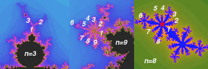
Recall that, for every rational number $\textstyle\frac{p}{q}$ , where p and q are relatively prime, there is a hyperbolic component of period q bifurcating from the main cardioid. The part of the Mandelbrot set connected to the main cardioid at this bifurcation point is called the p/q-limb. Computer experiments suggest that the diameter of the limb tends to zero like $\textstyle\frac{1}{q^2}$ . The best current estimate known is the famous Yoccoz-inequality, which states that the size tends to zero like $\textstyle\frac{1}{q}$ .

A period-q limb will have q − 1 "antennae" at the top of its limb. We can thus determine the period of a given bulb by counting these antennas.

[edit] Image gallery of a zoom sequence

The Mandelbrot set shows more intricate detail the closer one looks or magnifies the image, usually called "zooming in". The following example of an image sequence zooming to a selected c value gives an impression of the infinite richness of different geometrical structures, and explains some of their typical rules.

The magnification of the last image relative to the first one is about 10,000,000,000 to 1. Relating to an ordinary monitor, it represents a section of a Mandelbrot set with a diameter of 4 million kilometres. Its border would show an inconceivable number of different fractal structures.

Start	Step 1	Step 2	Step 3	Step 4
Step 5	Step 6	Step 7	Step 8	Step 9
Step 10	Step 11	Step 12	Step 13	Step 14

Start: Mandelbrot set with continuously coloured environment.

Gap between the "head" and the "body" also called the "seahorse valley".
On the left double-spirals, on the right "seahorses".
"Seahorse" upside down, its "body" is composed by 25 "spokes" consisting of 2 groups of 12 "spokes" each and one "spoke" connecting to the main cardioid; these 2 groups can be attributed by some kind of metamorphosis to the 2 "fingers" of the "upper hand" of the Mandelbrot set, therefore, the number of "spokes" increases from one "seahorse" to the next by 2; the "hub" is a so-called Misiurewicz point; between the "upper part of the body" and the "tail" a distorted small copy of the Mandelbrot set called satellite may be recognized.
The central endpoint of the "seahorse tail" is also a Misiurewicz point.
Part of the "tail" — there is only one path consisting of the thin structures that leads through the whole "tail"; this zigzag path passes the "hubs" of the large objects with 25 "spokes" at the inner and outer border of the "tail"; it makes sure that the Mandelbrot set is a so-called simply connected set, which means there are no islands and no loop roads around a hole.
Satellite. The two "seahorse tails" are the beginning of a series of concentric crowns with the satellite in the center.
Each of these crowns consists of similar "seahorse tails"; their number increases with powers of 2, a typical phenomenon in the environment of satellites, the unique path to the spiral center mentioned in zoom step 5 passes the satellite from the groove of the cardioid to the top of the "antenna" on the "head".
"Antenna" of the satellite. Several satellites of second order may be recognized.
The "seahorse valley" of the satellite. All the structures from the image of zoom step 1 reappear.
Double-spirals and "seahorses" - unlike the image of zoom step 2 they have appendices consisting of structures like "seahorse tails"; this demonstrates the typical linking of n+1 different structures in the environment of satellites of the order n, here for the simplest case n=1.
Double-spirals with satellites of second order - analog to the "seahorses" the double-spirals may be interpreted as a metamorphosis of the "antenna".
In the outer part of the appendices islands of structures may be recognized; they have a shape like Julia sets J_c; the largest of them may be found in the center of the "double-hook" on the right side.
Part of the "double-hook".
At first sight, these islands seem to consist of infinitely many parts like Cantor sets, as is actually the case for the corresponding Julia set J_c. Here they are connected by tiny structures so that the whole represents a simply connected set. These tiny structures meet each other at a satellite in the center that is too small to be recognized at this magnification. The value of c for the corresponding J_c is not that of the image center but, relative to the main body of the Mandelbrot set, has the same position as the center of this image relative to the satellite shown in zoom step 7.

[edit] Zoom animation

Mandelbrot set inward zoom of the above image gallery. 64-bit floating point numbers won't allow a deeper zoom than this.

Regardless of the extent to which one zooms in on a Mandelbrot set, there is always additional detail to see. During the twelve-second zoom in the animation at left, the set becomes magnified eleven-million fold. Thus, assuming the first frame is life-size at 45 mm across, a carbon atom would comprise 36 pixels in the final frame.

[edit] Generalizations

For general families of holomorphic functions, the boundary of the Mandelbrot set generalizes to the bifurcation locus, which is a natural object to study even when the connectedness locus is not useful.

Multibrot sets are bounded sets found in the complex plane for members of the general monic univariate polynomial family of recursions

$z \mapsto z^d + c.\$

[edit] Other non-analytic mappings

Of particular interest is the tricorn fractal, the connectedness locus of the anti-holomorphic family

$z \mapsto \bar{z}^2 + c\, .$

The tricorn (also sometimes called the Mandelbar set) was encountered by Milnor in his study of parameter slices of real cubic polynomials. It is not locally connected. This property is inherited by the connectedness locus of real cubic polynomials.

Another non-analytic generalization is the Burning Ship fractal which is obtained by iterating the mapping

$z \mapsto (|\Re \left(z\right)|+i|\Im \left(z\right)|)^2 + c\, .$

Multibrot set with d changing from 0 to 7

Multibrot sets of degrees 3 and 4

The tricorn fractal

The Burning Ship fractal

The Multibrot set is obtained by varying the value of the exponent d. The video shows its development from d = 0 to 7 at which point there are 6 i.e. (d - 1) lobes around the perimeter. A similar development with negative exponents results in d+1 clefts on the inside of a ring.

[edit] Computer drawings

Buddhabrot method

Still image of a movie of increasing magnification on 0.001643721971153 + 0.822467633298876i

Algorithms:

Escape time algorithm
- boolean version (draws M-set and its exterior using 2 colours) — Mandelbrot algorithm
- discrete (integer) version — level set method (LSM/M); draws Mandelbrot set and colour bands in its exterior
- continuous version
- level curves version — draws lemniscates of Mandelbrot set — boundaries of Level Sets^[16]
- decomposition of exterior of Mandelbrot set
complex potential
- Hubbard-Douady (real) potential of Mandelbrot set (CPM/M) - radial part of complex potential
- external angle of Mandelbrot set — angular part of complex potential
- abstract M-set
Distance estimation method for Mandelbrot set
- exterior distance estimation — Milnor algorithm (DEM/M)
- interior distance estimation
algorithm used to explore interior of Mandelbrot set
- period of hyperbolic components
- multiplier of periodic orbit (internal rays(angle) and internal radius)
- bof61 and bof60

Every algorithm can be implemented in sequential or parallel version. Mirror symmetry can be used to speed-up calculations.

[edit] Escape time algorithm

The simplest algorithm for generating a representation of the Mandelbrot set is known as the "escape time" algorithm. A repeating calculation is performed for each x, y point in the plot area and based on the behaviour of that calculation, a colour is chosen for that pixel.

The x and y locations of each point are used as starting values in a repeating, or iterating calculation (described in detail below). The result of each iteration is used as the starting values for the next. The values are checked during each iteration to see if they have reached a critical 'escape' condition or 'bailout'. If that condition is reached, the calculation is stopped, the pixel is drawn, and the next x, y point is examined. For some starting values, escape occurs quickly, after only a small number of iterations. For starting values very close to but not in the set, it may take hundreds or thousands of iterations to escape. For values within the Mandelbrot set, escape will never occur. The programmer or user must choose how much iteration, or 'depth,' they wish to examine. The higher the maximum number of iterations, the more detail and subtlety emerge in the final image, but the longer time it will take to calculate the fractal image.

Escape conditions can be simple or complex. Because no complex number with a real or imaginary part greater than 2 can be part of the set, a common bailout is to escape when either coefficient exceeds 2. A more computationally complex method, but which detects escapes sooner, is to compute the distance from the origin using the Pythagorean theorem, and if this distance exceeds two, the point has reached escape. More computationally-intensive rendering variations such as Buddhabrot detect an escape, then use values iterated along the way.

The colour of each point represents how quickly the values reached the escape point. Often black is used to show values that fail to escape before the iteration limit, and gradually brighter colours are used for points that escape. This gives a visual representation of how many cycles were required before reaching the escape condition.

[edit] For programmers

The definition of the Mandelbrot set, together with its basic properties, suggests a simple algorithm for drawing a picture of the Mandelbrot set. The region of the complex plane we are considering is subdivided into a certain number of pixels. To color any such pixel, let $c$ be the midpoint of that pixel. We now iterate the critical value $c$ under $P c$ , checking at each step whether the orbit point has modulus larger than 2.

If this is the case, we know that the midpoint does not belong to the Mandelbrot set, and we color our pixel. (Either we color it white to get the simple mathematical image or color it according to the number of iterations used to get the well-known colorful images). Otherwise, we keep iterating for a certain (large, but fixed) number of steps, after which we decide that our parameter is "probably" in the Mandelbrot set, or at least very close to it, and color the pixel black.

In pseudocode, this algorithm would look as follows.

For each pixel on the screen do:
{
  x = x0 = x co-ordinate of pixel
  y = y0 = y co-ordinate of pixel

  iteration = 0
  max_iteration = 1000
 
  while ( x*x + y*y <= (2*2)  AND  iteration < max_iteration ) 
  {
    xtemp = x*x - y*y + x0
    y = 2*x*y + y0

    x = xtemp

    iteration = iteration + 1
  }
 
  if ( iteration == max_iteration ) 
  then 
    color = black
  else 
    color = iteration

  plot(x0,y0,color)
}

where, relating the pseudocode to $c$ , $z$ and $P c$ :

$z = x + i y$
$z 2 = x 2 + i 2 x y - y 2$
$c = x 0 + i y 0$

and so, as can be seen in the pseudocode in the computation of x and y:

$x = \mathop{\mathrm{Re}}(z^2+c) = x^2-y^2+\mathit{x0}$ and y = $\mathop{\mathrm{Im}}(z^2+c) = 2xy+\mathit{y0}$

To get colorful images of the set, the assignment of a color to each value of the number of executed iterations can be made using one of a variety of functions (linear, exponential, etc). One practical way to do it, without slowing down the calculations, is to use the number of executed iterations as an entry to a look-up color palette table initialized at startup. If the color table has, for instance, 500 entries, then you can use n mod 500, where n is the number of iterations, to select the color to use. You can initialize the color palette matrix in various different ways, depending on what special feature of the escape behavior you want to emphasize graphically.

[edit] Continuous (smooth) coloring

This image was rendered with the Escape Time Algorithm. Notice the very obvious "bands" of color.

This image was rendered with the Normalized Iteration Count Algorithm. Notice the bands of color have been replaced by a smooth gradient.

Another example of the Normalized Iteration Count Algorithm. Notice that there is no banding effect; all of the colors flow into each other. Also, the colors take on the same pattern that would be observed if the Escape Time Algorithm was used.

The Escape Time Algorithm is popular for its simplicity. However, it creates bands of color, which, as a type of aliasing can detract from an image's aesthetic value. This can be improved using the Normalized Iteration Count Algorithm,^[17] which provides a smooth transition of colors between iterations. The algorithm associates a real number $ν$ with each value of z using the equation

$\nu(z,B,P)=n+\frac{\ln(2\ln(B))-\ln(\ln(|z_n|))}{\ln(P)}\,$ ,

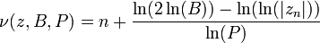where n is the number of iterations for z to escape, z_n is the value after n iterations, B is the bailout radius (normally 2 for a Mandelbrot set, but it can be changed), and P is the power for which z is raised to in the Mandelbrot set equation (z_n+1 = z_n^P + c, P is generally 2). Another formula for this is

$\nu(z)=\lim\limits_{n\to\infty}n-\log_2\log_2|z_n|\ .$

Note that this new formula is simpler than the first, but it requies a large bailout radius and doesn't work for generalized Mandelbrot sets.
While this algorithm is relatively simple to implement (using either formula), there are a few things that need to be taken into consideration. First, the two formulae return a continuous stream of numbers. However, it is up to the programmer to decide on how the return values will be converted into a color. Some type of method for casting these numbers onto a gradient should be developed. Second, it is recommended that a few extra iterations are done so that z can grow. If iterations cease as soon as z escapes, there is the possibility that the smoothing algorithm will not work.

[edit] Distance estimates

One can compute distance from point c (in exterior or interior) to nearest point on the boundary of Mandelbrot set.^[18]

[edit] Exterior distance estimation

The proof of the connectedness of the Mandelbrot set in fact gives a formula for the uniformizing map of the complement of $M$ (and the derivative of this map). By the Koebe 1/4 theorem, one can then estimate the distance between the mid-point of our pixel and the Mandelbrot set up to a factor of 4.

In other words, provided that the maximal number of iterations is sufficiently high, one obtains a picture of the Mandelbrot set with the following properties:

Every pixel which contains a point of the Mandelbrot set is colored black.
Every pixel which is colored black is close to the Mandelbrot set.

Exterior distance estimate may be used to color whole complement of Mandelbrot set

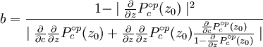
The distance estimate of a pixel c (a complex number) from the Mandelbrot set is given by

$b=\lim_{n \to \infty} 2\cdot\ln(\mid{P_c^{\circ n}(c)}\mid)\cdot\frac{\mid{P_c^{\circ n}(c)}\mid}{\mid\frac{\partial}{\partial{c}} P_c^{\circ n}(c)\mid}$

where

$P_c(z) \,$ stands for complex quadratic polynomial
$P_c^{\circ n}(c)$ stands for n iterations of $P_c(z) \to z$ or $z^2 + c \to z$ , starting with z=c: $P_c^{\circ 0}(c) = c$ , $P_c^{\circ n+1}(c) = P_c^{\circ n}(c)^2 + c$ ;
$\frac{\partial}{\partial{c}} P_c^{\circ n}(c)$ is the derivative of $P_c^{\circ n}(c)$ with respect to c. This derivative can be found by starting with $\frac{\partial}{\partial{c}} P_c^{\circ 0}(c) = 1$ and then $\frac{\partial}{\partial{c}} P_c^{\circ n+1}(c) = 2\cdot{}P_c^{\circ n}(c)\cdot\frac{\partial}{\partial{c}} P_c^{\circ n}(c) + 1$ . This can easily be verified by using the chain rule for the derivative.

From a mathematician's point of view, this formula only works in limit where n goes to infinity, but very reasonable estimates can be found with just a few additional iterations after the main loop exits.

Once b is found, by the Koebe 1/4-theorem, we know there's no point of the Mandelbrot set with distance from c smaller than b/4.

[edit] Interior distance estimation

Pixels colored according to the estimated interior distance

It is also possible to estimate the distance of a limitly periodic (i.e., inner) point to the boundary of the Mandelbrot set. The estimate is given by

$b=\frac{1-\mid{\frac{\partial}{\partial{z}}P_c^{\circ p}(z_0)}\mid^2} {\mid{\frac{\partial}{\partial{c}}\frac{\partial}{\partial{z}}P_c^{\circ p}(z_0) + \frac{\partial}{\partial{z}}\frac{\partial}{\partial{z}}P_c^{\circ p}(z_0) \frac{\frac{\partial}{\partial{c}}P_c^{\circ p}(z_0)} {1-\frac{\partial}{\partial{z}}P_c^{\circ p}(z_0)}}\mid}$

where

$p$ is the period,
$c$ is the point to be estimated,
$P c (z)$ is the complex quadratic polynomial $P c (z) = z 2 + c$
$P_c^{\circ p}(z_0)$ is $p$ compositions of $P_c(z) \to z$ , starting with $P_c^{\circ 0}(z) = z_0$
$z 0$ is any of the $p$ points that make the attractor of the iterations of $P_c(z) \to z$ starting with $P_c^{\circ 0}(z) = c$ ; $z 0$ satisfies $z_0 = P_c^{\circ p}(z_0)$ ,
$\frac{\partial}{\partial{c}}\frac{\partial}{\partial{z}}P_c^{\circ p}(z_0)$ , $\frac{\partial}{\partial{z}}\frac{\partial}{\partial{z}}P_c^{\circ p}(z_0)$ , $\frac{\partial}{\partial{c}}P_c^{\circ p}(z_0)$ and $\frac{\partial}{\partial{z}}P_c^{\circ p}(z_0)$ are various derivatives of $P_c^{\circ p}(z)$ , evaluated at $z 0$ .

Given $p$ and $z 0$ , $P_c^{\circ p}(z_0)$ and its derivatives can be evaluated by:

$\begin{align} \frac{\partial}{\partial{c}}\frac{\partial}{\partial{z}}P_c^{\circ 0}(z_0) = & 0 \\ \frac{\partial}{\partial{z}}\frac{\partial}{\partial{z}}P_c^{\circ 0}(z_0) = & 0 \\ \frac{\partial}{\partial{c}}P_c^{\circ 0}(z_0) = & 0 \\ \frac{\partial}{\partial{z}}P_c^{\circ 0}(z_0) = & 1 \\ P_c^{\circ 0}(z_0) = & z_0\end{align}$
$\begin{align} \frac{\partial}{\partial{c}}\frac{\partial}{\partial{z}}P_c^{\circ n+1}(z_0) & = 2\cdot(\frac{\partial}{\partial{c}}P_c^{\circ n}(z_0) \cdot\frac{\partial}{\partial{z}}P_c^{\circ n}(z_0) + P_c^{\circ n}(z_0)\cdot\frac{\partial}{\partial{c}}\frac{\partial}{\partial{z}}P_c^{\circ n}(z_0)) \\ \frac{\partial}{\partial{z}}\frac{\partial}{\partial{z}}P_c^{\circ n+1}(z_0) & = 2\cdot(\frac{\partial}{\partial{z}}P_c^{\circ n}(z_0)^2 + P_c^{\circ n}(z_0)\cdot \frac{\partial}{\partial{z}}\frac{\partial}{\partial{z}}P_c^{\circ n}(z_0)) \\ \frac{\partial}{\partial{c}}P_c^{\circ n+1}(z_0) & = 2\cdot P_c^{\circ n}(z_0)\cdot\frac{\partial}{\partial{c}}P_c^{\circ n}(z_0) + 1 \\ \frac{\partial}{\partial{z}}P_c^{\circ n+1}(z_0) & = 2\cdot P_c^{\circ n}(z_0)\cdot\frac{\partial}{\partial{z}}P_c^{\circ n}(z_0) \\ P_c^{\circ n+1}(z_0) & = P_c^{\circ n}(z_0)^2 + c\end{align}$ .

Analogous to the exterior case, once b is found, we know that all points within the distance of b/4 from c are inside the Mandelbrot set.

There are two practical problems with the interior distance estimate: first, we need to find $z 0$ precisely, and second, we need to find $p$ precisely. The problem with $z 0$ is that the convergence to $z 0$ by iterating $P c (z)$ requires, theoretically, an infinite number of operations. The problem with period is that, sometimes, due to rounding errors, a period is falsely identified to be an integer multiple of the real period (e.g., a period of 86 is detected, while the real period is only 43=86/2). In such case, the distance is overestimated, i.e., the reported radius could contain points outside the Mandelbrot set.

3D view : smallest absolute value of the orbit of the interior points of the Mandelbrot set

[edit] Optimizations

One way to improve calculations is to find out beforehand whether the given point lies within the cardioid or in the period-2 bulb.

To prevent having to do huge numbers of iterations for other points in the set, one can do "periodicity checking"—which means check if a point reached in iterating a pixel has been reached before. If so, the pixel cannot diverge, and must be in the set. This is most relevant for fixed-point calculations, where there is a relatively high chance of such periodicity—a full floating-point (or higher-accuracy) implementation would rarely go into such a period.

Periodicity checking is, of course, a trade-off: The need to remember points costs memory and data management instructions, whereas it saves computational instructions.

[edit] Popular Culture

The Jonathan Coulton song, "Mandelbrot Set", is a tribute to both the fractal itself, and its creator Benoît Mandelbrot. A video by a Cornell University student used the song to also pay homage to the mathematician. However, his description of the generation of a Mandelbrot Set is actually one of a Julia Set.
In The Ghost from the Grand Banks by Arthur C. Clarke, the Craig family is obsessed with Mandelbrot set, even having a pond in its shape dug. However Clarke's descriptions of the M-set are wrong.^[19]

[edit] See also

[edit] References

^ "Mandelbrot Set Explorer: Mathematical Glossary". http://math.bu.edu/DYSYS/explorer/def.html. Retrieved on 2007-10-07.
^ Robert Brooks and Peter Matelski, The dynamics of 2-generator subgroups of PSL(2,C), in "Riemann Surfaces and Related Topics", ed. Kra and Maskit, Ann. Math. Stud. 97, 65–71, ISBN 0-691-08264-2
^ Benoît Mandelbrot, Fractal aspects of the iteration of $z\mapsto\lambda z(1-z)$ for complex $λ, z$ , Annals NY Acad. Sci. 357, 249/259
^ Adrien Douady and John H. Hubbard, Etude dynamique des polynômes complexes, Prépublications mathémathiques d'Orsay 2/4 (1984 / 1985)
^ Peitgen, Heinz-Otto; Richter Peter (1986). The Beauty of Fractals. Heidelberg: Springer-Verlag. ISBN 0-387-15851-0.
^ Frontiers of Chaos, Exhibition of the Goethe-Institut by H.O. Peitgen, P. Richter, H. Jürgens, M. Prüfer, D.Saupe. since 1985 shown in over 40 countries.
^ Glieck, James (1987). Chaos: Making a New Science. London: Cardinal. pp. 229.
^ Dewdney, A.K. (Aug1985). A computer microscope zooms in for a close look at the most complicated object in mathematics. Scientific American. pp. 16–24.
^ Fractals: The Patterns of Chaos. John Briggs. 1992. p. 80.
^ Lyubich, Mikhail (May-June, 1999). Six Lectures on Real and Complex Dynamics. http://citeseer.ist.psu.edu/cache/papers/cs/28564/http:zSzzSzwww.math.sunysb.eduzSz~mlyubichzSzlectures.pdf/. Retrieved on 2007-04-04.
^ Lyubich, Mikhail (November 1998). "Regular and stochastic dynamics in the real quadratic family" (PDF). Proceedings of the National Academy of Sciences of the United States of America 95: 14025–14027. doi:10.1073/pnas.95.24.14025. PMID 9826646. http://www.pnas.org/cgi/reprint/95/24/14025.pdf. Retrieved on 2007-04-04.
^ http://www.mrob.com/pub/muency/pixelcounting.html
^ Lei.pdf Tan Lei, "Similarity between the Mandelbrot set and Julia Sets", Communications in Mathematical Physics 134 (1990), pp. 587-617.
^ J. Milnor, "Self-Similarity and Hairiness in the Mandelbrot Set", in Computers in Geometry and Topology, M. Tangora (editor), Dekker, New York, pp. 211-257.
^ Mitsuhiro Shishikura, The Hausdorff dimension of the boundary of the Mandelbrot set and Julia sets, Ann. of Math. 147 (1998) p. 225-267. (First appeared in 1991 as a Stony Brook IMS Preprint, available as arXiv:math.DS/9201282.)
^ M. Romera, G. Pastor, and F. Montoya (1996). "Drawing the Mandelbrot set by the method of the escape lines". Fractalia 5 (No. 17): 11–13. http://www.iec.csic.es/~miguel/Preprint3.ps.
^ García, Francisco; Ángel Fernández, Javier Barrallo, Luis Martín (PDF). Coloring Dynamical Systems in the Complex Plane. http://math.unipa.it/~grim/Jbarrallo.PDF. Retrieved on 2008-01-21.
^ Albert Lobo Cusidó. "Interior and exterior distance bounds for the Mandelbrot". http://usuarios.lycos.es/llopsite/BuddhaBrotA2.htm.
^ Kasman, Alex. "MathFiction: The Ghost from the Grand Banks (Arthur C. Clarke)". http://math.cofc.edu/kasman/MATHFICT/mfview.php?callnumber=mf12. Retrieved on 2008-11-05.

[edit] Further reading

Lennart Carleson and Theodore W. Gamelin, Complex Dynamics, Springer 1993, ISBN 0-387-97942-5
John W. Milnor, Dynamics in One Complex Variable (Third Edition), Annals of Mathematics Studies 160, Princeton University Press 2006, ISBN 0-691-12488-4 (First appeared in 1990 as a Stony Brook IMS Preprint, available as arXiV:math.DS/9201272.)
Nigel Lesmoir-Gordon. "The Colours of Infinity: The Beauty, The Power and the Sense of Fractals." ISBN 1-904555-05-5 (The book comes with a related DVD of the Arthur C. Clarke documentary introduction to the fractal concept and the Mandelbrot set, with music by David Gilmour, of the progressive rock band Pink Floyd).
Heinz-Otto Peitgen, Hartmut Jürgens, Dietmar Saupe: Chaos and Fractals - New Frontiers of Science, Springer, New-York 1992,2004. ISBN 0-387-20229-3

[edit] External links

Wikimedia Commons has media related to: Mandelbrot set

Wikibooks has a book on the topic of

Fractals

[0] "Mandelbrot Set Explorer: Mathematical Glossary". http://math.bu.edu/DYSYS/explorer/def.html. Retrieved on 2007-10-07.

[1] Robert Brooks and Peter Matelski, The dynamics of 2-generator subgroups of PSL(2,C), in "Riemann Surfaces and Related Topics", ed. Kra and Maskit, Ann. Math. Stud. 97, 65–71, ISBN 0-691-08264-2

[2] Benoît Mandelbrot, Fractal aspects of the iteration of $z\mapsto\lambda z(1-z)$ for complex $λ, z$ , Annals NY Acad. Sci. 357, 249/259

[3] Adrien Douady and John H. Hubbard, Etude dynamique des polynômes complexes, Prépublications mathémathiques d'Orsay 2/4 (1984 / 1985)

[4] Peitgen, Heinz-Otto; Richter Peter (1986). The Beauty of Fractals. Heidelberg: Springer-Verlag. ISBN 0-387-15851-0.

[5] Frontiers of Chaos, Exhibition of the Goethe-Institut by H.O. Peitgen, P. Richter, H. Jürgens, M. Prüfer, D.Saupe. since 1985 shown in over 40 countries.

[6] Glieck, James (1987). Chaos: Making a New Science. London: Cardinal. pp. 229.

[7] Dewdney, A.K. (Aug1985). A computer microscope zooms in for a close look at the most complicated object in mathematics. Scientific American. pp. 16–24.

[8] Fractals: The Patterns of Chaos. John Briggs. 1992. p. 80.

[9] Lyubich, Mikhail (May-June, 1999). Six Lectures on Real and Complex Dynamics. http://citeseer.ist.psu.edu/cache/papers/cs/28564/http:zSzzSzwww.math.sunysb.eduzSz~mlyubichzSzlectures.pdf/. Retrieved on 2007-04-04.

[10] Lyubich, Mikhail (November 1998). "Regular and stochastic dynamics in the real quadratic family" (PDF). Proceedings of the National Academy of Sciences of the United States of America 95: 14025–14027. doi:10.1073/pnas.95.24.14025. PMID 9826646. http://www.pnas.org/cgi/reprint/95/24/14025.pdf. Retrieved on 2007-04-04.

[11] ttp://www.mrob.com/pub/muency/pixelcounting.html

[12] Lei.pdf Tan Lei, "Similarity between the Mandelbrot set and Julia Sets", Communications in Mathematical Physics 134 (1990), pp. 587-617.

[13] J. Milnor, "Self-Similarity and Hairiness in the Mandelbrot Set", in Computers in Geometry and Topology, M. Tangora (editor), Dekker, New York, pp. 211-257.

[14] Mitsuhiro Shishikura, The Hausdorff dimension of the boundary of the Mandelbrot set and Julia sets, Ann. of Math. 147 (1998) p. 225-267. (First appeared in 1991 as a Stony Brook IMS Preprint, available as arXiv:math.DS/9201282.)

[15] M. Romera, G. Pastor, and F. Montoya (1996). "Drawing the Mandelbrot set by the method of the escape lines". Fractalia 5 (No. 17): 11–13. http://www.iec.csic.es/~miguel/Preprint3.ps.

[16] García, Francisco; Ángel Fernández, Javier Barrallo, Luis Martín (PDF). Coloring Dynamical Systems in the Complex Plane. http://math.unipa.it/~grim/Jbarrallo.PDF. Retrieved on 2008-01-21.

[17] Albert Lobo Cusidó. "Interior and exterior distance bounds for the Mandelbrot". http://usuarios.lycos.es/llopsite/BuddhaBrotA2.htm.

[18] Kasman, Alex. "MathFiction: The Ghost from the Grand Banks (Arthur C. Clarke)". http://math.cofc.edu/kasman/MATHFICT/mfview.php?callnumber=mf12. Retrieved on 2008-11-05.

[1]

[2]

[3]

[4]

[5]

[6]

[7]

[8]

[9]

[10]

[11]

[12]

[13]

[14]

[15]

[16]

[17]

[18]

[19]