Logistic function

From Wikipedia, the free encyclopedia

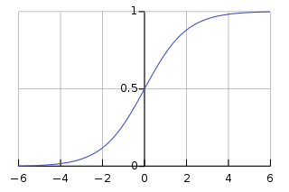
Standard logistic sigmoid function

A logistic function or logistic curve is the most common sigmoid curve. It models the S-curve of growth of some set^[1] P, where P might be thought of as population. The initial stage of growth is approximately exponential; then, as saturation begins, the growth slows, and at maturity, growth stops.

A simple^[2] logistic function may be defined by the formula

$P(t) = \frac{1}{1 + e^{-t}} \!$

where the variable^[3] P might be considered to denote a population and the variable t might be thought of as time. If we now let $t$ range over the real numbers from $-\infty$ to $+\infty$ then we obtain the S-curve shown. In practice, due to the nature of the exponential function $e - t$ , it is sufficient to compute t over a small range of real numbers such as $[ - 6, + 6]$ .

The logistic function finds applications in a range of fields, including artificial neural networks, biology, biomathematics, demography, economics, chemistry, mathematical psychology, probability, sociology and statistics.

1 Logistic differential equation
2 In ecology: modeling population growth
- 2.1 Time-varying carrying capacity
3 In neural networks
4 In statistics
5 In medicine: modeling of growth of tumors
6 In chemistry: reaction models
7 In physics: Fermi distribution
8 Double logistic function
9 See also
10 Notes
11 References
12 External links

[edit] Logistic differential equation

The logistic function is the solution of the simple^[2] first-order non-linear differential equation

$\frac{dP}{dt}=P(1-P) \!$

where P is a variable^[3] with respect to time t and with boundary condition P(0) = 1/2. This equation is the continuous version of the logistic map. One may readily find the (symbolic) solution to be

$P(t)=\frac{e^{t}}{e^{t}+e^{c}}$

Choosing the constant of integration $e c = 1$ gives the other well-known form of the definition of the logistic curve

$P(t) = \frac{e^{t}}{1 + e^{t}} \!$

The logistic curve shows early exponential growth for negative t, which slows to linear growth of slope 1/4 near t = 0, then approaches y = 1 with an exponentially decaying gap.

The logistic function is the inverse of the natural logit function and so can be used to convert the logarithm of odds into a probability; the conversion from the log-likelihood ratio of two alternatives also takes the form of a logistic curve.

The logistic sigmoid function is related to the hyperbolic tangent, A.p. by

$2 \, P(t) = 1 + \tanh \left( \frac{t}{2} \right).$

[edit] In ecology: modeling population growth

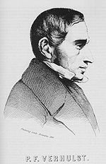
Pierre-François Verhulst (1804-1849)

A typical application of the logistic equation^[4] is a common model of population growth, originally due to Pierre-François Verhulst in 1838, where the rate of reproduction is proportional to:

the existing population,
the amount of available resources

all else being equal. Thus the second term models the competition for available resources, which tends to limit the population growth. Letting P represent population size (N is often used in ecology instead) and t represent time, this model is formalized by the differential equation:

$\frac{dP}{dt}=rP\left(1 - \frac{P}{K}\right)$

where the constant r defines the growth rate and K is the carrying capacity.

Interpreting the equation shown above: the early, unimpeded growth rate is modeled by the first term +rP. The value of the rate r represents the proportional increase of the population P in one unit of time. Later, as the population grows, the second term, which multiplied out is −rP²/K, becomes larger than the first as some members of the population P interfere with each other by competing for some critical resource, such as food or living space. This antagonistic effect is called the bottleneck, and is modelled by the value of the parameter K. The competition diminishes the combined growth rate, until the value of P ceases to grow (this is called maturity of the population).

Let us divide both sides of the equation by K^[5] to give

$\frac{d}{dt}\frac{P}{K}=r\frac{P}{K}\left(1 - \frac{P}{K}\right)$

Now setting $x = P / K$ gives us the differential equation

$\frac{dx}{dt} = r x (1-x)$

For $r = 1$ we have the particular case with which we started.

In ecology, species are sometimes referred to as r-strategist or K-strategist depending upon the selective processes that have shaped their life history strategies. The solution to the equation (with $P 0$ being the initial population) is

$P(t) = \frac{K P_0 e^{rt}}{K + P_0 \left( e^{rt} - 1\right)}$

where

$\lim_{t\to\infty} P(t) = K.\,$

Which is to say that K is the limiting value of P: the highest value that the population can reach given infinite time (or come close to reaching in finite time). It is important to stress that the carrying capacity is asymptotically reached independently of the initial value P(0) > 0, also in case that P(0) > K.

[edit] Time-varying carrying capacity

Since the environmental conditions influences the carrying capacity, as a consequence it can be time-varying: K(t) > 0, leading to the following mathematical model:

$\frac{dP}{dt}=rP\left(1 - \frac{P}{K(t)}\right)$

A particularly important case is that of carrying capacity that varies periodically with period T:

$K(t+T) = K(t).\,$

It can be shown that in such a case, independently from the initial value P(0) > 0, P(t) will tend to a unique periodic solution P_*(t), whose period is T.

A typical value of T is one year: in such case K(t) reflects periodical variations of weather conditions.

[edit] In neural networks

Logistic functions are often used in neural networks to introduce nonlinearity in the model and/or to clamp signals to within a specified range. A popular neural net element computes a linear combination of its input signals, and applies a bounded logistic function to the result; this model can be seen as a "smoothed" variant of the classical threshold neuron.

A common choice for the activation or "squashing" functions, used to clip for large magnitudes to keep the response of the neural network bounded^[6] is

$g(h) = \frac{1}{1 + e^{-2 \beta h}} \!$

which we recognize to be of the form of the logistic function. These relationships result in simplified implementations of artificial neural networks with artificial neurons.

[edit] In statistics

Logistic functions are used in several roles in statistics. Firstly, they are the cumulative distribution function of the logistic family of distributions. Secondly they are used in logistic regression to model how the probability p of an event may be affected by one or more explanatory variables: an example would be to have the model

$p=P(a + bx)\,$

where x is the explanatory variable and a and b are model parameters to be fitted.

An important application of the logistic function is in the Rasch model, used in item response theory. In particular, the Rasch model forms a basis for maximum likelihood estimation of the locations of objects or persons on a continuum, based on collections of categorical data, for example the abilities of persons on a continuum based on responses that have been categorized as correct and incorrect.

[edit] In medicine: modeling of growth of tumors

Another application of logistic curve is in medicine, where the logistic differential equation is used to model the growth of tumors. This application can be considered an extension of the above mentioned use in the framework of ecology. Denoting with X(t) the size of the tumor at time t, its dynamics is governed by:

$X^{\prime}=r\left(1 - \frac{X}{K}\right)X$

which is of the type:

$X^{\prime}=F\left(X\right)X$

where F(X) is the proliferation rate of the tumor.

If a chemotherapy is started with a log-kill effect, the equation may be revised to be

$X^{\prime}=r\left(1 - \frac{X}{K}\right)X - c(t)X,$

where c(t) is the therapy-induced death rate. In the idealized case of very long therapy, c(t) can be modeled as a periodic function (of period T) or (in case of continuous infusion therapy) as a constant function, and one has that

$\frac{1}{T}\int_{0}^{T}{c(t)\, dt} > r \Rightarrow \lim_{t \rightarrow +\infty }x(t)=0$

i.e. if the average therapy-induced death rate is greater than the baseline proliferation rate then there is the eradication of the disease. Of course, this is an over-simplified model of both the growth and the therapy (e.g. it does not take into account the phenomenon of clonal resistance).

[edit] In chemistry: reaction models

Concentration of reactants and products in autocatalytical reactions follow the logistic function.

[edit] In physics: Fermi distribution

Determines the statistical distribution of fermions over the energy states for a system in thermal equilibrium. In other words, it is the distribution of the probabilities that each possible energy levels is occupied by a fermion, according to Fermi-Dirac statistics.

[edit] Double logistic function

Double logistic sigmoid curve

The double logistic is a function similar to the logistic function with numerous applications. Its general formula is:

$y = \mbox{sgn}(x-d) \, \Bigg(1-\exp\bigg(-\bigg(\frac{x-d}{s}\bigg)^2\bigg)\Bigg),$

where d is its centre and s is the steepness factor. Here "sgn" represents the sign function.

It is based on the Gaussian curve and graphically it is similar to two identical logistic sigmoids bonded together at the point x = d.

One of its applications is non-linear normalization of a sample, as it has the property of eliminating outliers.

[edit] See also

[edit] Notes

^ set: Here P denotes a set. Later we will use P to denote a function which varies over time. Normally such a function is written P(t). However, such a function may also be read as a set of ordered pairs of the form <t, P(t)>. By convention mathematicians are wont to write P to denote such a set.
^ ^a ^b simple: The word simple is used here in a technical sense. There are many different varieties of the form of the logistic function. This is true for most mathematical objects. We will notice the same phenomenon with respect to the corresponding logistic differential equation. It is good practice to begin with a simple form which shows the nature of the mathematical object in question.
^ ^a ^b variable: When we speak of the variable P we usually think of it as a function of the variable t which denotes time. Hence, wherever we write P we are using a conventional shorthand for P(t) to say that P varies over time.
^ The Verhulst equation was first published by Pierre-François Verhulst in 1838 after he had read Thomas Malthus' An Essay on the Principle of Population. Verhulst derived his logistic equation to describe the self-limiting growth of a biological population. The equation is also sometimes called the Verhulst-Pearl equation following its rediscovery in 1920. Alfred J. Lotka derived the equation again in 1925, calling it the law of population growth.
^ Eric Weisstein at Wolfram Research
^ Gershenfeld 1999, p.150

[edit] References

Gershenfeld, Neil (1999), The Nature of Mathematical Modeling, Cambridge, UK.: Cambridge University Press, ISBN 978-0521-570954
Kingsland, S. E. (1995) Modeling nature ISBN 0-226-43728-0
Weisstein, Eric W. "Logistic Equation". From MathWorld--A Wolfram Web Resource. http://mathworld.wolfram.com/LogisticEquation.html. Retrieved on 2008-10-21.

[edit] External links

[set-0] set: Here P denotes a set. Later we will use P to denote a function which varies over time. Normally such a function is written P(t). However, such a function may also be read as a set of ordered pairs of the form <t, P(t)>. By convention mathematicians are wont to write P to denote such a set.

[simple-1] simple: The word simple is used here in a technical sense. There are many different varieties of the form of the logistic function. This is true for most mathematical objects. We will notice the same phenomenon with respect to the corresponding logistic differential equation. It is good practice to begin with a simple form which shows the nature of the mathematical object in question.

[variable-2] variable: When we speak of the variable P we usually think of it as a function of the variable t which denotes time. Hence, wherever we write P we are using a conventional shorthand for P(t) to say that P varies over time.

[Verhulst_equation-3] The Verhulst equation was first published by Pierre-François Verhulst in 1838 after he had read Thomas Malthus' An Essay on the Principle of Population. Verhulst derived his logistic equation to describe the self-limiting growth of a biological population. The equation is also sometimes called the Verhulst-Pearl equation following its rediscovery in 1920. Alfred J. Lotka derived the equation again in 1925, calling it the law of population growth.

[Weisstein_at_MathWorld-4] Eric Weisstein at Wolfram Research

[Gershenfeld-1999-5] Gershenfeld 1999, p.150

[1]

[2]

[3]

[4]

[5]

[6]

Logistic function

From Wikipedia, the free encyclopedia

Contents

[edit] Logistic differential equation

[edit] In ecology: modeling population growth

[edit] Time-varying carrying capacity

[edit] In neural networks

[edit] In statistics

[edit] In medicine: modeling of growth of tumors

[edit] In chemistry: reaction models

[edit] In physics: Fermi distribution

[edit] Double logistic function

[edit] See also

[edit] Notes

[edit] References

[edit] External links

Views

Personal tools

Navigation

Search

Interaction

Toolbox

Languages