Calculus
From Wikipedia, the free encyclopedia
Calculus (Latin, calculus, a small stone used for counting) is a branch of mathematics that includes the study of limits, derivatives, integrals, and infinite series, and constitutes a major part of modern university education. Historically, it has been referred to as "the calculus of infinitesimals", or "infinitesimal calculus". Most basically, calculus is the study of change, in the same way that geometry is the study of space.
Calculus has widespread applications in science, economics, and engineering and is used to solve problems for which algebra alone is insufficient. Calculus builds on algebra, trigonometry, and analytic geometry and includes two major branches, differential calculus and integral calculus, that are related by the fundamental theorem of calculus. In more advanced mathematics, calculus is usually called analysis and is defined as the study of functions.
More generally, calculus (plural calculi) may refer to any method or system of calculation guided by the symbolic manipulation of expressions. Some examples of other well-known calculi are propositional calculus, predicate calculus, relational calculus, and lambda calculus.
Contents |
[edit] History

[edit] Ancient
The ancient period introduced some of the ideas of integral calculus, but does not seem to have developed these ideas in a rigorous or systematic way. Calculating volumes and areas, the basic function of integral calculus, can be traced back to the Egyptian Moscow papyrus (c. 1820 BC), in which an Egyptian successfully calculated the volume of a pyramidal frustum.[1][2] From the school of Greek mathematics, Eudoxus (c. 408−355 BC) used the method of exhaustion, which prefigures the concept of the limit, to calculate areas and volumes while Archimedes (c. 287−212 BC) developed this idea further, inventing heuristics which resemble integral calculus.[3] The method of exhaustion was later used in China by Liu Hui in the 3rd century AD in order to find the area of a circle. The Cavalieri's Theorem was used by Zu Chongzhi in the 5th century AD, who used it to find the volume of a sphere.[2]
[edit] Medieval
Around AD 1000, the Islamic mathematician, Ibn al-Haytham (Alhacen), was the first to derive the formula for the sum of the fourth powers of an arithmetic progression, using a method that is readily generalizable to finding the formula for the sum of any higher integral powers, which he used to perform an integration.[4] In the 11th century, the Chinese polymath Shen Kuo developed 'packing' equations that dealt with integration. In the 12th century, the Indian mathematician, Bhāskara II, developed an early derivative representing infinitesimal change, and he described an early form of "Rolle's theorem".[5] Also in the 12th century, the Persian mathematician Sharaf al-Dīn al-Tūsī discovered the derivative of cubic polynomials, an important result in differential calculus.[6] In the 14th century, Madhava of Sangamagrama, along with other mathematician-astronomers of the Kerala school of astronomy and mathematics, described special cases of Taylor series,[7] which are treated in the text Yuktibhasa.[8][9][10]
[edit] Modern
In the modern period, independent discoveries relating to calculus were being made in early 17th century Japan, by mathematicians such as Seki Kowa, who expanded upon the method of exhaustion.
In Europe, the foundational work was a treatise due to Bonaventure Cavaliers, who argued that volumes and areas should be computed as the sums of the volumes and areas of infinitesimal thin cross-sections. The ideas were similar to Archimedes' in The Method, but this treatise was lost until the early part of the twentieth century. Cavalier's work was not well respected, and the infinitesimal quantities he introduced were disreputable at first.
The formal study of calculus combined Cavalier's infinitesimals with the calculus of finite differences developed in Europe at around the same time. The combination was achieved by John Wallis, Isaac Barrow, and James Gregory, the latter two proving the second fundamental theorem of calculus around 1675.
The product rule and chain rule, the notion of higher derivatives, Taylor series, and analytical were introduced by Isaac Newton in an idiosyncratic notation which he used to solve problems of mathematical physics. In his publications, Newton rephrased his ideas to suit the mathematical idiom of the time, replacing calculations with infinitesimals by equivalent geometrical arguments which were considered beyond reproach. He used the methods of calculus to solve the problem of planetary motion, the shape of the surface of a rotating fluid, the oblateness of the earth, the motion of a weight sliding on a cycloid, and many other problems discussed in his Principia Mathematica. In other work, he developed series expansions for functions, including fractional and irrational powers, and it was clear that he understood the principles of the Taylor series. He did not publish all these discoveries, and at this time infinitesimal methods were still considered disreputable.

These ideas were systematized into a true calculus of infinitesimals by Gottfried Wilhelm Leibniz, who was originally accused of plagiarism by Newton. He is now regarded as an independent inventor of and contributor to calculus. His contribution was to provide a clear set of rules for manipulating infinitesimal quantities, allowing the computation of second and higher derivatives, and providing the product rule and chain rule, in their differential and integral forms. Unlike Newton, Leibniz paid a lot of attention to the formalism--- he often spent days determining appropriate symbols for concepts.
Leibniz and Newton are usually both credited with the invention of calculus. Newton was the first to apply calculus to general physics and Leibniz developed much of the notation used in calculus today. The basic insights that both Newton and Leibniz provided were the laws of differentiation and integration, second and higher derivatives, and the notion of an approximating polynomial series. By Newton's time, the fundamental theorem of calculus was known.
When Newton and Leibniz first published their results, there was great controversy over which mathematician (and therefore which country) deserved credit. Newton derived his results first, but Leibniz published first. Newton claimed Leibniz stole ideas from his unpublished notes, which Newton had shared with a few members of the Royal Society. This controversy divided English-speaking mathematicians from continental mathematicians for many years, to the detriment of English mathematics. A careful examination of the papers of Leibniz and Newton shows that they arrived at their results independently, with Leibniz starting first with integration and Newton with differentiation. Today, both Newton and Leibniz are given credit for developing calculus independently. It is Leibniz, however, who gave the new discipline its name. Newton called his calculus "the science of fluxions".
Since the time of Leibniz and Newton, many mathematicians have contributed to the continuing development of calculus. In the 19th century, calculus was put on a much more rigorous footing by mathematicians such as Cauchy, Riemann, and Weierstrass (see (ε, δ)-definition of limit). It was also during this period that the ideas of calculus were generalized to Euclidean space and the complex plane. Lebesgue generalized the notion of the integral so that pretty much any function has an integral, while Laurent Schwartz extended differentiation in much the same way.
Calculus is a ubiquitous topic in most modern high schools and universities, and mathematicians around the world continue to contribute to its development.[11]
[edit] Significance
While some of the ideas of calculus were developed earlier in Greece, China, India, Iraq, Persia, and Japan, the modern use of calculus began in Europe, during the 17th century, when Isaac Newton and Gottfried Wilhelm Leibniz built on the work of earlier mathematicians to introduce its basic principles. The development of calculus was built on earlier concepts of instantaneous motion and area underneath curves.
Applications of differential calculus include computations involving velocity and acceleration, the slope of a curve, and optimization. Applications of integral calculus include computations involving area, volume, arc length, center of mass, work, and pressure. More advanced applications include power series and Fourier series. Calculus can be used to compute the trajectory of a shuttle docking at a space station or the amount of snow in a driveway.
Calculus is also used to gain a more precise understanding of the nature of space, time, and motion. For centuries, mathematicians and philosophers wrestled with paradoxes involving division by zero or sums of infinitely many numbers. These questions arise in the study of motion and area. The ancient Greek philosopher Zeno gave several famous examples of such paradoxes. Calculus provides tools, especially the limit and the infinite series, which resolve the paradoxes.
[edit] Foundations
In mathematics, foundations refers to the rigorous development of a subject from precise axioms and definitions. Working out a rigorous foundation for calculus occupied mathematicians for much of the century following Newton and Leibniz and is still to some extent an active area of research today.
There is more than one rigorous approach to the foundation of calculus. The usual one today is via the concept of limits defined on the continuum of real numbers. An alternative is nonstandard analysis, in which the real number system is augmented with infinitesimal and infinite numbers, as in the original Newton-Leibniz conception. The foundations of calculus are included in the field of real analysis, which contains full definitions and proofs of the theorems of calculus as well as generalizations such as measure theory and distribution theory.
[edit] Principles
[edit] Limits and infinitesimals
Calculus is usually developed by manipulating very small quantities. Historically, the first method of doing so was by infinitesimals. These are objects which can be treated like numbers but which are, in some sense, "infinitely small". An infinitesimal number dx could be greater than 0, but less than any number in the sequence 1, 1/2, 1/3, ... and less than any positive real number. Any integer multiple of an infinitesimal is still infinitely small, i.e., infinitesimals do not satisfy the Archimedean property. From this point of view, calculus is a collection of techniques for manipulating infinitesimals. This approach fell out of favor in the 19th century because it was difficult to make the notion of an infinitesimal precise. However, the concept was revived in the 20th century with the introduction of non-standard analysis and smooth infinitesimal analysis, which provided solid foundations for the manipulation of infinitesimals.
In the 19th century, infinitesimals were replaced by limits. Limits describe the value of a function at a certain input in terms of its values at nearby input. They capture small-scale behavior, just like infinitesimals, but use the ordinary real number system. In this treatment, calculus is a collection of techniques for manipulating certain limits. Infinitesimals get replaced by very small numbers, and the infinitely small behavior of the function is found by taking the limiting behavior for smaller and smaller numbers. Limits are easy to put on rigorous foundations, and for this reason they are usually considered to be the standard approach to calculus.
[edit] Differential calculus

Differential calculus is the study of the definition, properties, and applications of the derivative or slope of a function. The process of finding the derivative is called differentiation. In technical language, the derivative is a linear operator, which inputs a function and outputs a second function, so that at every point the value of the output is the slope of the input.
The concept of the derivative is fundamentally more advanced than the concepts encountered in algebra. In algebra, students learn about functions which input a number and output another number. For example, if the doubling function inputs 3, then it outputs 6, while if the squaring function inputs 3, it outputs 9. But the derivative inputs a function and outputs another function. For example, if the derivative inputs the squaring function, then it outputs the doubling function, because the doubling function gives the slope of the squaring function at any given point.
To understand the derivative, students must learn mathematical notation. In mathematical notation, one common symbol for the derivative of a function is an apostrophe-like mark called prime. Thus the derivative of f is f′ (spoken "f prime"). The last sentence of the preceding paragraph, in mathematical notation, would be written

If the input of a function is time, then the derivative of that function is the rate at which the function changes.
If a function is linear (that is, if the graph of the function is a straight line), then the function can be written y = mx + b, where:
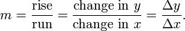
This gives an exact value for the slope of a straight line. If the graph of the function is not a straight line, however, then the change in y divided by the change in x varies, and we can use calculus to find an exact value at a given point. (Note that y and f(x) represent the same thing: the output of the function. This is known as function notation.) A line through two points on a curve is called a secant line. The slope, or rise over run, of a secant line can be expressed as

where the coordinates of the first point are (x, f(x)) and h is the horizontal distance between the two points.
To determine the slope of the curve, we use the limit:

Working out one particular case, we find the slope of the squaring function at the point where the input is 3 and the output is 9 (i.e., f(x) = x2, so f(3) = 9).
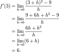
The slope of the squaring function at the point (3,9) is 6, that is to say, it is going up six times as fast as it is going to the right.
The limit process just described can be generalized to any point on the graph of any function. The procedure can be visualized as in the following figure.

Here the function involved (drawn in red) is f(x) = x3 − x. The tangent line (in green) which passes through the point (−3/2, −15/8) has a slope of 23/4. Note that the vertical and horizontal scales in this image are different.
[edit] Leibniz notation
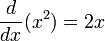
A common notation, introduced by Leibniz, for the derivative in the example above is

In an approach based on limits, the symbol dy/dx is to be interpreted not as the quotient of two numbers but as a shorthand for the limit computed above. Leibniz, however, did intend it to represent the quotient of two infinitesimally small numbers, dy being the infinitesimally small change in y caused by an infinitesimally small change dx applied to x. We can also think of d/dx as a differentiation operator, which takes a function as an input and gives another function, the derivative, as the output. For example:
In this usage, the dx in the denominator is read as "with respect to x." Even when calculus is developed using limits rather than infinitesimals, it is common to manipulate symbols like dx and dy as if they were real numbers; although it is possible to avoid such manipulations, they are sometimes notationally convenient in expressing operations such as the total derivative.
[edit] Integral calculus
Integral calculus is the study of the definitions, properties, and applications of two related concepts, the indefinite integral and the definite integral. The process of finding the value of an integral is called integration. In technical language, integral calculus studies two related linear operators.
The indefinite integral is the antiderivative, the inverse operation to the derivative. F is an indefinite integral of f when f is a derivative of F. (This use of upper- and lower-case letters for a function and its indefinite integral is common in calculus.)
The definite integral inputs a function and outputs a number, which gives the area between the graph of the input and the x-axis. The technical definition of the definite integral is the limit of a sum of areas of rectangles, called a Riemann sum.
A motivating example is the distances traveled in a given time.

If the speed is constant, only multiplication is needed, but if the speed changes, then we need a more powerful method of finding the distance. One such method is to approximate the distance traveled by breaking up the time into many short intervals of time, then multiplying the time elapsed in each interval by one of the speeds in that interval, and then taking the sum (a Riemann sum) of the approximate distance traveled in each interval. The basic idea is that if only a short time elapses, then the speed will stay more or less the same. However, a Riemann sum only gives an approximation of the distance traveled. We must take the limit of all such Riemann sums to find the exact distance traveled.

If f(x) in the diagram on the left represents speed as it varies over time, the distance traveled (between the times represented by a and b) is the area of the shaded region s.
To approximate that area, an intuitive method would be to divide up the distance between a and b into a number of equal segments, the length of each segment represented by the symbol Δx. For each small segment, we can choose one value of the function f(x). Call that value h. Then the area of the rectangle with base Δx and height h gives the distance (time Δx multiplied by speed h) traveled in that segment. Associated with each segment is the average value of the function above it, f(x)=h. The sum of all such rectangles gives an approximation of the area between the axis and the curve, which is an approximation of the total distance traveled. A smaller value for Δx will give more rectangles and in most cases a better approximation, but for an exact answer we need to take a limit as Δx approaches zero.
The symbol of integration is  , an elongated S (the S stands for "sum"). The definite integral is written as:

and is read "the integral from a to b of f-of-x with respect to x." The Leibniz notation dx is intended to suggest dividing the area under the curve into an infinite number of rectangles, so that their width Δx becomes the infinitesimally small dx. In a formulation of the calculus based on limits, the notation  is to be understood as an operator that takes a function as an input and gives a number, the area, as an output; dx is not a number, and is not being multiplied by f(x).
The indefinite integral, or antiderivative, is written:

Functions differing by only a constant have the same derivative, and therefore the antiderivative of a given function is actually a family of functions differing only by a constant. Since the derivative of the function y = x² + C, where C is any constant, is y′ = 2x, the antiderivative of the latter is given by:
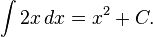
An undetermined constant like C in the antiderivative is known as a constant of integration.
[edit] Fundamental theorem
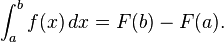
The fundamental theorem of calculus states that differentiation and integration are inverse operations. More precisely, it relates the values of antiderivatives to definite integrals. Because it is usually easier to compute an antiderivative than to apply the definition of a definite integral, the Fundamental Theorem of Calculus provides a practical way of computing definite integrals. It can also be interpreted as a precise statement of the fact that differentiation is the inverse of integration.
The Fundamental Theorem of Calculus states: If a function f is continuous on the interval [a, b] and if F is a function whose derivative is f on the interval (a, b), then
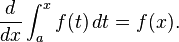
Furthermore, for every x in the interval (a, b),
This realization, made by both Newton and Leibniz, who based their results on earlier work by Isaac Barrow, was key to the massive proliferation of analytic results after their work became known. The fundamental theorem provides an algebraic method of computing many definite integrals—without performing limit processes—by finding formulas for antiderivatives. It is also a prototype solution of a differential equation. Differential equations relate an unknown function to its derivatives, and are ubiquitous in the sciences.
[edit] Applications
Calculus is used in every branch of the physical sciences, in computer science, statistics, engineering, economics, business, medicine, demography, and in other fields wherever a problem can be mathematically modeled and an optimal solution is desired.
Physics makes particular use of calculus; all concepts in classical mechanics are interrelated through calculus. The mass of an object of known density, the moment of inertia of objects, as well as the total energy of an object within a conservative field can be found by the use of calculus. In the subfields of electricity and magnetism calculus can be used to find the total flux of electromagnetic fields. A more historical example of the use of calculus in physics is Newton's second law of motion, it expressly uses the term "rate of change" which refers to the derivative: The rate of change of momentum of a body is equal to the resultant force acting on the body and is in the same direction. Even the common expression of Newton's second law as Force = Mass × Acceleration involves differential calculus because acceleration can be expressed as the derivative of velocity. Maxwell's theory of electromagnetism and Einstein's theory of general relativity are also expressed in the language of differential calculus. Chemistry also uses calculus in determining reaction rates and radioactive decay.
Calculus can be used in conjunction with other mathematical disciplines. For example, it can be used with linear algebra to find the "best fit" linear approximation for a set of points in a domain.
Green's Theorem, which gives the relationship between a line integral around a simple closed curve C and a double integral over the plane region D bounded by C, is applied in an instrument known as a planimeter which is used to calculate the area of a flat surface on a drawing. For example, it can be used to calculate the amount of area taken up by an irregularly shaped flower bed or swimming pool when designing the layout of a piece of property.
In the realm of medicine, calculus can be used to find the optimal branching angle of a blood vessel so as to maximize flow.
In analytic geometry, the study of graphs of functions, calculus is used to find high points and low points (maxima and minima), slope, concavity and inflection points.
In economics, calculus allows for the determination of maximal profit by providing a way to easily calculate both marginal cost and marginal revenue.
Calculus can be used to find approximate solutions to equations, in methods such as Newton's method, fixed point iteration, and linear approximation. For instance, spacecraft use a variation of the Euler method to approximate curved courses within zero gravity environments.
[edit] See also
[edit] Lists
- List of basic calculus topics
- List of basic calculus equations and formulas
- List of calculus topics
- Publications in calculus
- Table of integrals
[edit] Related topics
- Calculus with polynomials
- Complex analysis
- Differential equation
- Differential geometry
- Elementary calculus
- Fourier series
- Integral equation
- Mathematical analysis
- Mathematics
- Multivariable calculus
- Non-classical analysis
- Non-standard analysis
- Non-standard calculus
- Precalculus (mathematical education)
- Product Integrals
- Stochastic calculus
- Taylor series
[edit] References
[edit] Notes
- ^ There is no exact evidence on how it was done; some, including Morris Kline (Mathematical thought from ancient to modern times Vol. I) suggest trial and error.
- ^ a b Helmer Aslaksen. Why Calculus? National University of Singapore.
- ^ Archimedes, Method, in The Works of Archimedes ISBN 978-0-521-66160-7
- ^ Victor J. Katz (1995). "Ideas of Calculus in Islam and India", Mathematics Magazine 68 (3), pp. 163-174.
- ^ Ian G. Pearce. Bhaskaracharya II.
- ^ J. L. Berggren (1990). "Innovation and Tradition in Sharaf al-Din al-Tusi's Muadalat", Journal of the American Oriental Society 110 (2), pp. 304-309.
- ^ "Madhava". Biography of Madhava. School of Mathematics and Statistics University of St Andrews, Scotland. http://www-gap.dcs.st-and.ac.uk/~history/Biographies/Madhava.html. Retrieved on 2006-09-13.
- ^ "An overview of Indian mathematics". Indian Maths. School of Mathematics and Statistics University of St Andrews, Scotland. http://www-history.mcs.st-andrews.ac.uk/HistTopics/Indian_mathematics.html. Retrieved on 2006-07-07.
- ^ "Science and technology in free India" (PDF). Government of Kerala — Kerala Call, September 2004. Prof.C.G.Ramachandran Nair. http://www.kerala.gov.in/keralcallsep04/p22-24.pdf. Retrieved on 2006-07-09.
- ^ Charles Whish (1835). Transactions of the Royal Asiatic Society of Great Britain and Ireland.
- ^ UNESCO-World Data on Education [1]
[edit] Books
- Donald A. McQuarrie (2003). Mathematical Methods for Scientists and Engineers, University Science Books. ISBN 9781891389245
- James Stewart (2002). Calculus: Early Transcendentals, 5th ed., Brooks Cole. ISBN 9780534393212
[edit] Other resources
[edit] Further reading
- Courant, Richard ISBN 978-3540650584 Introduction to calculus and analysis 1.
- Edmund Landau. ISBN 0-8218-2830-4 Differential and Integral Calculus, American Mathematical Society.
- Robert A. Adams. (1999). ISBN 978-0-201-39607-2 Calculus: A complete course.
- Albers, Donald J.; Richard D. Anderson and Don O. Loftsgaarden, ed. (1986) Undergraduate Programs in the Mathematics and Computer Sciences: The 1985-1986 Survey, Mathematical Association of America No. 7.
- John L. Bell: A Primer of Infinitesimal Analysis, Cambridge University Press, 1998. ISBN 978-0-521-62401-5. Uses synthetic differential geometry and nilpotent infinitesimals.
- Florian Cajori, "The History of Notations of the Calculus." Annals of Mathematics, 2nd Ser., Vol. 25, No. 1 (Sep., 1923), pp. 1-46.
- Leonid P. Lebedev and Michael J. Cloud: "Approximating Perfection: a Mathematician's Journey into the World of Mechanics, Ch. 1: The Tools of Calculus", Princeton Univ. Press, 2004.
- Cliff Pickover. (2003). ISBN 978-0-471-26987-8 Calculus and Pizza: A Math Cookbook for the Hungry Mind.
- Michael Spivak. (September 1994). ISBN 978-0-914098-89-8 Calculus. Publish or Perish publishing.
- Tom M. Apostol. (1967). ISBN 9780471000051 Calculus, Volume 1, One-Variable Calculus with an Introduction to Linear Algebra. Wiley.
- Tom M. Apostol. (1969). ISBN 9780471000075 Calculus, Volume 2, Multi-Variable Calculus and Linear Algebra with Applications. Wiley.
- Silvanus P. Thompson and Martin Gardner. (1998). ISBN 978-0-312-18548-0 Calculus Made Easy.
- Mathematical Association of America. (1988). Calculus for a New Century; A Pump, Not a Filter, The Association, Stony Brook, NY. ED 300 252.
- Thomas/Finney. (1996). ISBN 978-0-201-53174-9 Calculus and Analytic geometry 9th, Addison Wesley.
- Weisstein, Eric W. "Second Fundamental Theorem of Calculus." From MathWorld--A Wolfram Web Resource.
- Mejlbro, Leif. "Real functions" Selection of calculus books
[edit] Online books
- Crowell, B. (2003). "Calculus" Light and Matter, Fullerton. Retrieved 6 May 2007 from http://www.lightandmatter.com/calc/calc.pdf
- Garrett, P. (2006). "Notes on first year calculus" University of Minnesota. Retrieved 6 May 2007 from http://www.math.umn.edu/~garrett/calculus/first_year/notes.pdf
- Faraz, H. (2006). "Understanding Calculus" Retrieved 6 May 2007 from Understanding Calculus, URL http://www.understandingcalculus.com/ (HTML only)
- Keisler, H. J. (2000). "Elementary Calculus: An Approach Using Infinitesimals" Retrieved 6 May 2007 from http://www.math.wisc.edu/~keisler/keislercalc1.pdf
- Mauch, S. (2004). "Sean's Applied Math Book" California Institute of Technology. Retrieved 6 May 2007 from http://www.cacr.caltech.edu/~sean/applied_math.pdf
- Sloughter, Dan (2000). "Difference Equations to Differential Equations: An introduction to calculus". Retrieved 17 March 2009 from http://synechism.org/drupal/de2de/
- Stroyan, K.D. (2004). "A brief introduction to infinitesimal calculus" University of Iowa. Retrieved 6 May 2007 from http://www.math.uiowa.edu/~stroyan/InfsmlCalculus/InfsmlCalc.htm (HTML only)
- Strang, G. (1991). "Calculus" Massachusetts Institute of Technology. Retrieved 6 May 2007 from http://ocw.mit.edu/ans7870/resources/Strang/strangtext.htm
- Smith, William V. (2001). "The Calculus" Retrieved 4 July 2008 [2] (HTML only).
[edit] Web pages
- Eric W. Weisstein, Calculus at MathWorld.
- Topics on Calculus at PlanetMath.
- Calculus Made Easy (1914) by Silvanus P. ThompsonFull text in PDF
- The Online Calculus course for transfer, notes, video lectures, active forum at San Francisco State University by Professor Arek Goetz
- Calculus.org: The Calculus page at University of California, Davis — contains resources and links to other sites
- COW: Calculus on the Web at Temple University - contains resources ranging from pre-calculus and associated algebra
- Online Integrator (WebMathematica) from Wolfram Research
- The Role of Calculus in College Mathematics from ERICDigests.org
- OpenCourseWare Calculus from the Massachusetts Institute of Technology
- Infinitesimal Calculus — an article on its historical development, in Encyclopaedia of Mathematics, Michiel Hazewinkel ed. .
[edit] External links
![]() Textbooks from Wikibooks
Textbooks from Wikibooks
![]() Quotations from Wikiquote
Quotations from Wikiquote
![]() Source texts from Wikisource
Source texts from Wikisource
![]() Images and media from Commons
Images and media from Commons
![]() News stories from Wikinews
News stories from Wikinews
|
|||||

