Hypergeometric distribution
From Wikipedia, the free encyclopedia
| Probability mass function |
|
| Cumulative distribution function |
|
| Parameters | 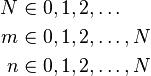 |
|---|---|
| Support |  |
| Probability mass function (pmf) |  |
| Cumulative distribution function (cdf) | |
| Mean |  |
| Median | |
| Mode | 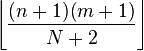 |
| Variance | 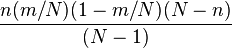 |
| Skewness | ![\frac{(N-2m)(N-1)^\frac{1}{2}(N-2n)}{[nm(N-m)(N-n)]^\frac{1}{2}(N-2)}](http://upload.wikimedia.org/math/c/b/c/cbc5d8105638f44a15bb6b6a42c98834.png) |
| Excess kurtosis | ![\left[\frac{N^2(N-1)}{n(N-2)(N-3)(N-n)}\right]](http://upload.wikimedia.org/math/b/5/c/b5c85bfac379f6390cf9ac846b3643cc.png)
|
| Entropy | |
| Moment-generating function (mgf) |  |
| Characteristic function | 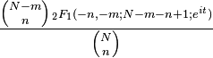 |

![+\left.\frac{3n(N-n)(N+6)}{N^2}-6\right]](http://upload.wikimedia.org/math/5/e/e/5eea883c0354dcf5301ca80d816a58c2.png)
In probability theory and statistics, the hypergeometric distribution is a discrete probability distribution that describes the number of successes in a sequence of n draws from a finite population without replacement, just as the binomial distribution describes the number of successes for draws with replacement.
A typical example is illustrated by this contingency table:
| drawn | not drawn | total | |
|---|---|---|---|
| defective | k | m − k | m |
| non-defective | n − k | N + k − n − m | N − m |
| total | n | N − n | N |
There is a shipment of N objects in which m are defective. The hypergeometric distribution describes the probability that exactly k objects are defective in a sample of n distinct objects drawn from the shipment.
In general, if a random variable X follows the hypergeometric distribution with parameters N, m and n, then the probability of getting exactly k "successes" (defective objects in the previous example) is given by

where the binomial coefficient  is defined to be the coefficient of xb in the polynomial expansion of (1 + x)a
The probability is positive when k is between max(0, n + m − N) and min(m, n).
The formula can be understood as follows: There are  possible samples (without replacement). There are
  ways to obtain k defective objects and there are
  ways to fill out the rest of the sample with non-defective objects.
The sum of the probabilities for all possible values of k is equal to 1 as one would expect intuitively; this is essentially Vandermonde's identity from combinatorics.
Contents |
[edit] Application and example
The classical application of the hypergeometric distribution is sampling without replacement. Think of an urn with two types of marbles, black ones and white ones. Define drawing a white marble as a success and drawing a black marble as a failure (analogous to the binomial distribution). If the variable N describes the number of all marbles in the urn (see contingency table above) and m describes the number of white marbles (called defective in the example above), then N − m corresponds to the number of black marbles.
Now, assume that there are 5 white and 45 black marbles in the urn. Standing next to the urn, you close your eyes and draw 10 marbles without replacement. What is the probability that exactly 4 of the 10 are white? Note that although we are looking at success/failure, the data cannot be modeled under the binomial distribution, because the probability of success on each trial is not the same, as the size of the remaining population changes as we remove each marble.
This problem is summarized by the following contingency table:
| drawn | not drawn | total | |
|---|---|---|---|
| white marbles | 4 (k) | 1 = 5 − 4 (m − k) | 5 (m) |
| black marbles | 6 = 10 − 4 (n − k) | 39 = 50 + 4 − 10 − 5 (N + k − n − m) | 45 (N − m) |
| total | 10 (n) | 40 (N − n) | 50 (N) |
The probability of drawing exactly k white marbles can be calculated by the formula

Hence, in this example k = 4, calculate

The probability of drawing exactly 4 white marbles is quite low, approximately 0.004, 4 in one thousand. If the random experiment of drawing 10 marbles from the urn of 50 marbles without replacement is repeated 1000 times, exactly 4 white ones would be drawn about 4 times.
Intuitively we would expect it to be even more unlikely for all 5 marbles to be white. The contingency table in this case is as follows:
| drawn | not drawn | total | |
|---|---|---|---|
| white marbles | 5 (k) | 0 = 5 − 5 (m − k) | 5 (m) |
| black marbles | 5 = 10 − 5 (n − k) | 40 = 50 + 5 − 10 − 5 (N + k − n − D) | 45 (N − m) |
| total | 10 (n) | 40 (N − n) | 50 (N) |
The probability is as follows (notice that the denominator is always the same):
![\Pr[K=5] = f(5;50,5,10) = {{{5 \choose 5} {{45} \choose {5}}}\over {50 \choose 10}} = 0.0001189375\dots,](http://upload.wikimedia.org/math/6/a/d/6add99251a3b365bf28644c77f4857bc.png)
As expected, the probability of drawing 5 white marbles is much lower than that of drawing 4.
[edit] Symmetries
- f(k;N,m,n) = f(n − k;N,N − m,n)
This symmetry can be intuitively understood if you repaint all the black marbles to white and vice versa, thus the black and white marbles simply change roles.
- f(k;N,m,n) = f(m − k;N,m,N − n)
This symmetry can be intuitively understood as swapping the roles of taken and not taken marbles.
- f(k;N,m,n) = f(k;N,n,m)
This symmetry can be intuitively understood if instead of drawing marbles, you label the marbles that you would have drawn. Both expressions give the probability that exactly k marbles are "black" and labeled "drawn".
[edit] Symmetric application
The metaphor of defective and drawn objects depicts an application of the hypergeometric distribution in which the interchange symmetry between n and m is not of foremost concern. Here is an alternate metaphor which brings this symmetry into sharper focus, as there are also applications where it serves no purpose to distinguish n from m.
Suppose you have a set of N children who have been identified with an unusual bone marrow antigen. The doctor wishes to conduct a heredity study to determine the inheritance pattern of this antigen. For the purposes of this study, the doctor wishes to draw tissue from the bone marrow from the biological mother and biological father of each child. This is an uncomfortable procedure, and not all the mothers and fathers will agree to participate. Of the mothers, m participate and N-m decline. Of the fathers, n participate and N-n decline.
We assume here that the decisions made by the mothers is independent of the decisions made by the fathers. Under this assumption, the doctor, who is given n and m, wishes to estimate k, the number of children where both parents have agreed to participate. The hypergeometric distribution can be used to determine this distribution over k. It's not straightforward why the doctor would know n and m, but not k. Perhaps n and m are dictated by the experimental design, while the experimenter is left blind to the true value of k.
It is important to recognize that for given N, n and m a single degree of freedom partitions N into four sub-populations:
1) Children where both parents participate
2) Children where only the mother participates
3) Children where only the father participates and
4) Children where neither parent participates.
Knowing any one of these four values determines the other three by simple arithmetic relations. For this reason, each of these quadrants is governed by an equivalent hypergeometric distribution. The mean, mode, and values of k contained within the support differ from one quadrant to another, but the size of the support, the variance, and other high order statistics do not.
For the purpose of this study, it might make no difference to the doctor whether the mother participates or the father participates. If this happens to be true, the doctor will view the result as a three-way partition: children where both parents participate, children where one parent participates, children where neither parent participates. Under this view, the last remaining distinction between n and m has been eliminated. The distribution where one parent participates is the sum of the distributions where either parent alone participates.
[edit] Symmetry and sampling
To express how the symmetry of the clinical metaphor degenerates to the asymmetry of the sampling language used in the drawn/defective metaphor, we will restate the clinical metaphor in the abstract language of decks and cards. We begin with a dealer who holds two prepared decks of N cards. The decks are labelled left and right. The left deck was prepared to hold n red cards, and N-n black cards; the right deck was prepared to hold m red cards, and N-m black cards.
These two decks are dealt out face down to form N hands. Each hand contains one card from the left deck and one card from the right deck. If we determine the number of hands that contain two red cards, by symmetry relations we will necessarily also know the hypergeometric distributions governing the other three quadrants: hand counts for red/black, black/red, and black/black. How many cards must be turned over to learn the total number of red/red hands? Which cards do we need to turn over to accomplish this? These are questions about possible sampling methods.
One approach is to begin by turning over the left card of each hand. For each hand showing a red card on the left, we then also turn over the right card in that hand. For any hand showing a black card on the left, we do not need to reveal the right card, as we already know this hand does not count toward the total of red/red hands. Our treatment of the left and right decks no longer appears symmetric: one deck was fully revealed while the other deck was partially revealed. However, we could just as easily have begun by revealing all cards dealt from the right deck, and partially revealed cards from the left deck.
In fact, the sampling procedure need not prioritize one deck over the other in the first place. Instead, we could flip a coin for each hand, turning over the left card on heads, and the right card on tails, leaving each hand with one card exposed. For every hand with a red card exposed, we reveal the companion card. This will suffice to allow us to count the red/red hands, even though under this sampling procedure neither the left nor right deck is fully revealed.
By another symmetry, we could also have elected to determine the number of black/black hands rather than the number of red/red hands, and discovered the same distributions by that method.
The symmetries of the hypergeometric distribution provide many options in how to conduct the sampling procedure to isolate the degree of freedom governed by the hypergeometric distribution. Even if the sampling procedure appears to treat the left deck differently from the right deck, or governs choices by red cards rather than black cards, it is important to recognize that the end result is essentially the same.
[edit] Relationship to Fisher's exact test
The test (see above) based on the hypergeometric distribution (hypergeometric test) is identical to the corresponding one-tailed version of Fisher's exact test. Reciprocally, the p-value of a two-sided Fisher's exact test can be calculated as the sum of two appropriate hypergeometric tests (for more information see [1]).
[edit] Related distributions
Let X ~ Hypergeometric(m, N, n) and p = m / N.
- If n = 1 then X has a Bernoulli distribution with parameter p.
- Let Y have a binomial distribution with parameters n and p; this models the number of successes in the analogous sampling problem with replacement. If N and m are large compared to n and p is not close to 0 or 1, then X and Y have similar distributions, i.e.,
![P[X \le k] \approx P[Y \le k]](http://upload.wikimedia.org/math/4/8/9/48940b1f37481d1c8f497f6290eec5e1.png) .
.
- If n is large, N and m are large compared to n and p is not close to 0 or 1, then
![P[X \le k] \approx \Phi \left( \frac{k-n p}{\sqrt{n p (1-p)}} \right)](http://upload.wikimedia.org/math/3/a/3/3a3b81ee8aa2bbd5b0351d65352ceeed.png)
where Φ is the standard normal distribution function
- If the probabilities to draw a white or red ball are not equal (e.g. because their size is different) then X has a Noncentral hypergeometric distribution
[edit] Multivariate hypergeometric distribution
| Probability mass function |
|
| Cumulative distribution function |
|
| Parameters |    ![n \in [0,N]](http://upload.wikimedia.org/math/e/2/b/e2b3fa1a6b8e27b6f8e91b7960c971e8.png) |
|---|---|
| Support |  |
| Probability mass function (pmf) |  |
| Cumulative distribution function (cdf) | |
| Mean | 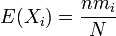 |
| Median | |
| Mode | |
| Variance | 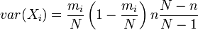  |
| Skewness | |
| Excess kurtosis | |
| Entropy | |
| Moment-generating function (mgf) | |
| Characteristic function | |
The model of an urn with black and white marbles can be extended to the case where there are more than two colors of marbles. If there are mi marbles of color i in the urn and you take n marbles at random without replacement, then the number of marbles of each color in the sample (k1,k2,...,kc) has the multivariate hypergeometric distribution.
The properties of this distribution are given in the adjacent table, where c is the number of different colors and  is the total number of marbles.
[edit] See also
- Binomial distribution
- Fisher's exact test
- Noncentral hypergeometric distributions
- Sampling (statistics)
- Urn problem
- Coupon collector's problem
- Geometric distribution
- Keno
[edit] References
- ^ K. Preacher and N. Briggs. "Calculation for Fisher's Exact Test: An interactive calculation tool for Fisher's exact probability test for 2 x 2 tables (interactive page)". http://www.people.ku.edu/~preacher/fisher/fisher.htm. Retrieved on 2008-04-08.
[edit] External links
- Hypergeometric Distribution Calculator
- Hypergeometric Distribution Calculator with source (Ruby, C++)
- The Hypergeometric Distribution and Binomial Approximation to a Hypergeometric Random Variable by Chris Boucher, Wolfram Demonstrations Project.
- Eric W. Weisstein, Hypergeometric Distribution at MathWorld.
- Hypergeometric distribution online calculater (.XBAP)
- Hypergeometric tail inequalities: ending the insanity by Matthew Skala.

