HSL and HSV
From Wikipedia, the free encyclopedia
|
|
This article needs additional citations for verification. Please help improve this article by adding reliable references (ideally, using inline citations). Unsourced material may be challenged and removed. (June 2007) |


HSL and HSV are two related representations of points in an RGB color space, which attempt to describe perceptual color relationships more accurately than RGB, while remaining computationally simple. HSL stands for hue, saturation, lightness, while HSV stands for hue, saturation, value.
HSI and HSB are alternative names for these concepts, using intensity and brightness; their definitions are less standardized, but they are typically interpreted as synonymous with HSL.
Both HSL and HSV describe colors as points in a cylinder whose central axis ranges from black at the bottom to white at the top with neutral colors between them, where angle around the axis corresponds to “hue”, distance from the axis corresponds to “saturation”, and distance along the axis corresponds to “lightness”, “value”, or “brightness”.
The two representations are similar in purpose, but differ somewhat in approach. Both are mathematically cylindrical, but while HSV (hue, saturation, value) can be thought of conceptually as an inverted cone of colors (with a black point at the bottom, and fully-saturated colors around a circle at the top), HSL conceptually represents a double-cone or sphere (with white at the top, black at the bottom, and the fully-saturated colors around the edge of a horizontal cross-section with middle gray at its center). Note that while “hue” in HSL and HSV refers to the same attribute, their definitions of “saturation” differ dramatically.
Because HSL and HSV are simple transformations of device-dependent RGB, the color defined by a (h, s, l) or (h, s, v) triplet depends on the particular color of red, green, and blue “primaries” used. Each unique RGB device therefore has unique HSL and HSV spaces to accompany it. An (h, s, l) or (h, s, v) triplet can however become definite when it is tied to a particular RGB color space, such as sRGB.
Both models were first formally described in 1978 by Alvy Ray Smith (though the concept of describing colors in three dimensions dates to the 18th century).[1][2]
Contents |
[edit] Motivation
It is sometimes preferable in working with art materials, digitized images, or other media, to use the HSV or HSL color model over alternative models such as RGB or CMYK, because of differences in the ways the models emulate how humans perceive color. RGB and CMYK are additive and subtractive models, respectively, modelling the way that primary color lights or pigments (respectively) combine to form new colors when mixed.
[edit] Usage

The HSV model is commonly used in computer graphics applications. In various application contexts, a user must choose a color to be applied to a particular graphical element. When used in this way, the HSV color wheel is often used. In it, the hue is represented by a circular region; a separate triangular region may be used to represent saturation and value. Typically, the vertical axis of the triangle indicates saturation, while the horizontal axis corresponds to value. In this way, a color can be chosen by first picking the hue from the circular region, then selecting the desired saturation and value from the triangular region.

Another visualization method of the HSV model is the cone. In this representation, the hue is depicted as a three-dimensional conical formation of the color wheel. The saturation is represented by the distance from the center of a circular cross-section of the cone, and the value is the distance from the pointed end of the cone. Some representations use a hexagonal cone, or hexcone, instead of a circular cone. This method is well-suited to visualizing the entire HSV color space in a single object; however, due to its three-dimensional nature, it is not well-suited to color selection in two-dimensional computer interfaces.
The HSV color space could also be visualized as a cylindrical object; similar to the cone above, the hue varies along the outer circumference of a cylinder, with saturation again varying with distance from the center of a circular cross-section. Value again varies from top to bottom. Such a representation might be considered the most mathematically accurate model of the HSV color space; however, in practice the number of visually distinct saturation levels and hues decreases as the value approaches black. Additionally, computers typically store RGB values with a limited range of precision; the constraints of precision, coupled with the limitations of human color perception, make the cone visualization more practical in most cases.
[edit] Comparison of HSL and HSV

HSL is similar to HSV. For some people, HSL better reflects the intuitive notion of "saturation" and "lightness" as two independent parameters, but for others its definition of saturation is wrong, as for example a very pastel, almost white color can be defined as fully saturated in HSL. It might be controversial, though, whether HSV or HSL is more suitable for use in human user interfaces.
The CSS3 specification from the W3C states, "Advantages of HSL are that it is symmetrical to lightness and darkness (which is not the case with HSV for example)…" This means that:
- In HSL, the Saturation component always goes from fully saturated color to the equivalent gray (in HSV, with V at maximum, it goes from saturated color to white, which may be considered counterintuitive).
- The Lightness in HSL always spans the entire range from black through the chosen hue to white (in HSV, the V component only goes half that way, from black to the chosen hue).
In software, a hue-based color model (HSV or HSL) is usually presented to the user in the form of a linear or circular hue chooser and a two-dimensional area (usually a square or a triangle) where the user can choose saturation and value/lightness for the selected hue. With this representation, the difference between HSV and HSL is irrelevant. However, many programs also let the user select a color via linear sliders or numeric entry fields, and for those controls, usually either HSL or HSV (not both) are used. HSV is traditionally more common. Here are some examples:

- Applications that use HSV (HSB):
- Apple Mac OS X system color picker (has a color disk for H/S and a slider for V)
- Xara Xtreme
- Adobe graphic applications (Illustrator, Photoshop, and others)
- PB MapInfo Pro
- Applications that use HSL:
- The CSS3 specification
- Inkscape (starting from version 0.42)
- Macromedia Studio
- Microsoft Windows system color picker (including Microsoft Paint)
- Paint Shop Pro
- ImageMagick
- Applications that use both HSV and HSL:
[edit] Comparison with other color models
The HSV tristimulus space does not technically support a one-to-one mapping to physical power spectra as measured in radiometry. Thus it is not generally advisable to try to make direct comparisons between HSV coordinates and physical light properties such as wavelength or amplitude.
| This section requires expansion. |
[edit] Formal specifications

|

|

|
HSL and HSV are defined mathematically by transformations between the r, g, and b coordinates of colors in RGB space and the h, s, l, and v coordinates of the HSL and HSV spaces.[3]
[edit] Conversion from RGB to HSL or HSV
Let r, g, b ∈ [0,1] be the red, green, and blue coordinates, respectively, of a color in RGB space.
Let max be the greatest of r, g, and b, and min the least.
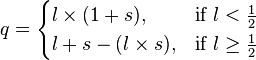
To find the hue angle h ∈ [0, 360] for either HSL or HSV space, compute:

To find saturation and lightness s, l ∈ [0,1] for HSL space, compute:


The value of h is generally normalized to lie between 0 and 360°, and h = 0 is used when max = min (that is, for grays) though the hue has no geometric meaning there, where the saturation s is zero. Similarly, the choice of 0 as the value for s when l is equal to 0 or 1 is arbitrary.
HSL and HSV have the same definition of hue, but the other components differ. The values for s and v of an HSV color are defined as follows:


The range of HSV and HSL vectors is a cube in the cartesian coordinate system; but since hue is really a cyclic property, it is not so necessary or appropriate to unwrap it, with a cut at 0 (red), into a linear coordinate. Therefore, visualizations of these spaces invariably involve hue circles;[4] cylindrical and conical (bi-conical for HSL) depictions are most popular; spherical depictions and other color solids are also possible.
[edit] Conversion from HSL to RGB
Given a color defined by (h, s, l) values in HSL space, with h in the range [0, 360), indicating the angle, in degrees of the hue, and with s and l in the range [0, 1], representing the saturation and lightness, respectively, a corresponding (r, g, b) triplet in RGB space, with r, g, and b also in range [0, 1], and corresponding to red, green, and blue, respectively, can be computed as follows:
First, if s = 0, then the resulting color is achromatic, or gray. In this special case, r, g, and b all equal l. Note that the value of h is ignored, and may be undefined in this situation.
The following procedure can be used, even when s is zero:

 (h normalized to be in the range [0,1))
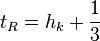

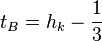


Compute each color component ColorC of the vector (ColorR, ColorG, ColorB) = (r, g, b),


[edit] Conversion from HSV to RGB
Similarly, given a color defined by (h, s, v) values in HSV space, with h as above, and with s and v varying between 0 and 1, representing the saturation and value, respectively, a corresponding (r, g, b) triplet in RGB space can be computed:


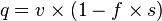
Compute color vector (r, g, b),

[edit] Terminology
The terms attributed to the "L" or "V" component of HSL or HSV color space may be misleading since they have little to do with color science definitions of the terms. In photometry, concepts such as lightness and luminance relate to a weighted spectrum, in which green is much more luminous than blue, and red is between; but in HSL and HSV, the "L" and "V" dimensions treat the three color channels equally.
- Lightness or value refers to the perceived reflectance of a surface,[5] or to relative luminous reflectance of a colored surface patch.
- Luminance typically refers to relative luminance, which is based on the photometric definition of luminance but normalized with respect to a reference white.
- Luminosity typically (and incorrectly) refers to relative luminance. This usage was popularized by Adobe Photoshop; in the documentation of the CS3 version, the luminosity blending mode is still present, but is described in terms of luminance: "Luminosity: Creates a result color with the hue and saturation of the base color and the luminance of the blend color."[6]
[edit] Spherical and other 3D mappings


HSL and HSV are related to three-dimensional color-order systems such as Philipp Otto Runge's color sphere (Farbenkugel) and the Munsell color system, both of which are structured around a neutral black-to-white axis, as the HSL and HSV cylinders are. Munsell refers to the colorfulness dimension as chroma rather than saturation, and refers to but uses hue and lightness as in HSL.
Modern works also sometimes map HSL into a sphere, with L along the polar axis, H a longitude, and S a fraction of the radius of the disk at a constant L or latitude.[7][8]
Since the entire top and bottom surfaces of the HSL cylinder are white and black, respectively, nothing is lost in shrinking them to points at the poles of a sphere. Another popular way to shrink the white and black surfaces to points is to map HSL to a bi-cone,[9][10] which fits the same description as the sphere given above, but with a different profile of radius versus L. For HSV, on the other hand, the top surface of the cylinder is not white, so it can not be collapsed to a point, while the bottom can be mapped to a point, since it's all black; therefore, HSV is commonly mapped to a cone.
|
|
Please help improve this section by expanding it. Further information might be found on the talk page. (February 2008) |
[edit] Examples
The RGB values are shown in the range 0.0 to 1.0.
| RGB | HSL | HSV | Result |
|---|---|---|---|
| (1, 0, 0) | (0°, 1, 0.5) | (0°, 1, 1) | |
| (0.5, 1, 0.5) | (120°, 1, 0.75) | (120°, 0.5, 1) | |
| (0, 0, 0.5) | (240°, 1, 0.25) | (240°, 1, 0.5) |
[edit] Notes
- ^ Alvy Ray Smith (August 1978). "Color Gamut Transform Pairs". Computer Graphics 12 (3): 12. doi:.
- ^ Kuehni, Rolf G. (February 2002). "The early development of the Munsell system". Color Research and Application 27 (1): 20–27. doi:..
- ^ Max K. Agoston (2005). Computer Graphics and Geometric Modeling: Implementation and Algorithms. Springer. ISBN 1852338180. http://books.google.com/books?id=fGX8yC-4vXUC&pg=PA303&dq=hsl+rgb+convert&lr=&as_brr=0&ei=aYOKR-nfEojuswOcoKDQBQ&sig=1s-pM0HzV34EeE8yb18RO64RVNE#PPA306,M1.
- ^ John C. Russ (2005). Image Analysis Of Food Microstructure. CRC Press. ISBN 0849322413. http://books.google.com/books?id=bY_eVN5PdJcC&pg=PA78&dq=HSL+cylinder+cone&lr=&as_brr=0&ei=A5-NR_fxBIOssgPY-MHQBQ&sig=9lrQJ5l1bKALtfWMwQur9LF0MGk.
- ^ Edward H. Adelson (2000). "Lightness Perception and Lightness Illusions – Some terminology". Massachusetts Institute of Technology. http://persci.mit.edu/people/adelson/publications/gazzan.dir/gazzan.htm#section4. Retrieved on 2007-07-17.
- ^ "List of Blending Modes". Adobe Help Resource Center. http://livedocs.adobe.com/en_US/Photoshop/10.0/help.html?content=WSfd1234e1c4b69f30ea53e41001031ab64-77e9.html. Retrieved on 2007-11-10.
- ^ Phil Nelson (2007). The Photographer's Guide to Color Management: Professional Techniques for Consistent Results. Amherst Media, Inc. ISBN 1584282045. http://books.google.com/books?id=CELdDlJ-Zj0C&pg=PT22&dq=hsl+sphere+color&lr=&as_brr=0&ei=OoGqR8OtMqPYiQGF3ejBCQ&sig=3PHf19l1beJtnrcOBVDP8bXQub0.
- ^ Abhay Sharma (2003). Understanding Color Management. Thomson Delmar Learning. ISBN 1401814476. http://books.google.com/books?id=KOyFSaUnNfMC&pg=PA79&dq=hsl+sphere+color&lr=&as_brr=0&ei=Bn-qR879LZ6GiQH85sSCBQ&sig=EOOhsvrOjw_GivtHU3j4AapVDHw.
- ^ John C. Russ (2005). Image Analysis Of Food Microstructure. CRC Press. ISBN 0849322413. http://books.google.com/books?id=bY_eVN5PdJcC&pg=PA77&dq=hue-saturation+bi-cone+color&lr=&as_brr=0&ei=ZYKqR63LF5XEigGR2sS5Cg&sig=D0k1BrWi3iHGsFpwbtDHJpZn2nE.
- ^ Richard Prikryl (2004). Dimension Stone 2004 - New Perspectives for a Traditional Building Material. Taylor & Francis. ISBN 9058096750. http://books.google.com/books?id=TDKI1V_Ph10C&pg=PA141&dq=hue-saturation++bi-conical+color&lr=&as_brr=0&ei=xoOqR8YiisyJAbLejYwB&sig=Fveiwwx3me4llIPitZ1gkjOTyqo#PPA141,M1.
[edit] References
- Raphael Gonzalez, Richard E. Woods (2002) Digital Image Processing, 2nd ed. Prentice Hall Press, ISBN 0-201-18075-8, p. 295.
- Charles Poynton. “What are HSB and HLS?” Color FAQ. 28 November 2006.
- Donald Hearn, M. Pauline Baker (1986) Computer Graphics. Prentice Hall International, ISBN 0-13-165598-1, pp. 302-205.
[edit] External links
- An explanation of HSL and how it differs from RGB can be found in the W3C's CSS3 Color Module.
- Formulas for converting to and from RGB can be found on EasyRGB.com.
- C++ code for RGB and HSV conversion
- Demonstrative color conversion applet
- HSV Colors by Hector Zenil, The Wolfram Demonstrations Project.
- HSV Tutorial in Basic, at The Mandelbrot Dazibao.
- HSL at CSS3 . Info very good and simple explanation of HSL
- An algorithm and code for performing HSV transformations directly on RGB colors
|
||||||||||||||||||||

