Derivative

	Topics in calculus
	Fundamental theorem; Limits of functions; Continuity; Vector calculus; Matrix calculus; Mean value theorem
	Differentiation
	Product rule; Quotient rule; Chain rule; Change of variables; Implicit differentiation; Taylor's theorem; Related rates; List of differentiation identities
	Integration
	Lists of integrals; Improper integrals; Integration by:; parts, disks, cylindrical; shells, substitution,; trigonometric substitution,; partial fractions, changing order

From Wikipedia, the free encyclopedia

Jump to: navigation, search

This article is about an overview of the term as used in calculus. For a non-technical overview of the subject, see Differential calculus. For other uses, see Derivative (disambiguation).

The graph of a function, drawn in black, and a tangent line to that function, drawn in red. The slope of the tangent line is equal to the derivative of the function at the marked point.

In calculus, a branch of mathematics, the derivative is a measure of how a function changes as its input changes. Loosely speaking, a derivative can be thought of as how much a quantity is changing at a given point. For example, the derivative of the position (or distance) of a vehicle with respect to time is the instantaneous velocity (respectively, instantaneous speed) at which the vehicle is traveling. Conversely, the integral of the velocity over time is the vehicle's position.

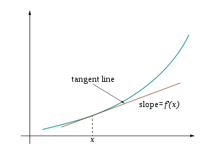
The derivative of a function at a chosen input value describes the best linear approximation of the function near that input value. For a real-valued function of a single real variable, the derivative at a point equals the slope of the tangent line to the graph of the function at that point. In higher dimensions, the derivative of a function at a point is a linear transformation called the linearization.^[1] A closely related notion is the differential of a function.

The process of finding a derivative is called differentiation. The fundamental theorem of calculus states that differentiation is the reverse process to integration.

[edit] Differentiation and the derivative

Click for larger image. At each point, the derivative of

f (x) = x * s i n (x 2) + 1

is the slope of a line that is tangent to the curve. The line is always tangent to the blue curve; its slope is the derivative. Note derivative is positive where green, negative where red, and zero where black.

Differentiation is a method to compute the rate at which a dependent output y, changes with respect to the change in the independent input x. This rate of change is called the derivative of y with respect to x. In more precise language, the dependence of y upon x means that y is a function of x. If x and y are real numbers, and if the graph of y is plotted against x, the derivative measures the slope of this graph at each point. This functional relationship is often denoted y = ƒ(x), where ƒ denotes the function.

The simplest case is when y is a linear function of x, meaning that the graph of y against x is a straight line. In this case, y = ƒ(x) = m x + c, for real numbers m and c, and the slope m is given by

$m={\mbox{change in } y \over \mbox{change in } x} = {\Delta y \over{\Delta x}}$

where the symbol Δ (the uppercase form of the Greek letter Delta) is an abbreviation for "change in." This formula is true because

y + Δy = ƒ(x+ Δx) = m (x + Δx) + c = m x + c + m Δx = y + mΔx.

It follows that Δy = m Δx.

This gives an exact value for the slope of a straight line. If the function ƒ is not linear (i.e. its graph is not a straight line), however, then the change in y divided by the change in x varies: differentiation is a method to find an exact value for this rate of change at any given value of x.

Figure 1. The tangent line at (x, ƒ(x))

Figure 2. The secant to curve y= ƒ(x) determined by points (x, ƒ(x)) and (x+h, ƒ(x+h)).

Figure 3. The tangent line as limit of secants.

The idea, illustrated by Figures 1-3, is to compute the rate of change as the limiting value of the ratio of the differences Δy / Δx as Δx becomes infinitely small.

In Leibniz's notation, such an infinitesimal change in x is denoted by dx, and the derivative of y with respect to x is written

$\frac{dy}{dx} \,\!$

suggesting the ratio of two infinitesimal quantities. (The above expression is read as "the derivative of y with respect to x", "d y by d x", or "d y over d x". The oral form "d y d x" is often used conversationally, although it may lead to confusion.)

The most common approach^[2] to turn this intuitive idea into a precise definition uses limits, but there are other methods, such as non-standard analysis.^[3]

[edit] Definition via difference quotients

Let ƒ be a real valued function. In classical geometry, the tangent line at a real number a was the unique line through the point (a, ƒ(a)) which did not meet the graph of ƒ transversally, meaning that the line did not pass straight through the graph. The derivative of y with respect to x at a is, geometrically, the slope of the tangent line to the graph of ƒ at a. The slope of the tangent line is very close to the slope of the line through (a, ƒ(a)) and a nearby point on the graph, for example (a + h, ƒ(a + h)). These lines are called secant lines. A value of h close to zero will give a good approximation to the slope of the tangent line, and smaller values (in absolute value) of h will, in general, give better approximations. The slope m of the secant line is the difference between the y values of these points divided by the difference between the x values, that is,

$m = \frac{\Delta f(x)}{\Delta x} = \frac{f(a+h)-f(a)}{h}.$

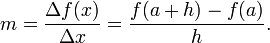
This expression is Newton's difference quotient. The derivative is the value of the difference quotient as the secant lines approach the tangent line. Formally, the derivative of the function ƒ at a is the limit

$f'(a)=\lim_{h\to 0}{f(a+h)-f(a)\over h}$

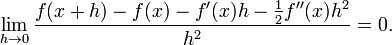
of the difference quotient as h approaches zero, if this limit exists. If the limit exists, then ƒ is differentiable at a. Here f′ (a) is one of several common notations for the derivative (see below).

Equivalently, the derivative satisfies the property that

$\lim_{h\to 0}{f(a+h)-f(a) - f'(a)\cdot h\over h} = 0,$

which has the intuitive interpretation (see Figure 1) that the tangent line to ƒ at a gives the best linear approximation

$f(a+h) \approx f(a) + f'(a)h$

to ƒ near a (i.e., for small h). This interpretation is the easiest to generalize to other settings (see below).

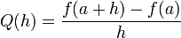
Substituting 0 for h in the difference quotient causes division by zero, so the slope of the tangent line cannot be found directly. Instead, define Q(h) to be the difference quotient as a function of h:

$Q(h) = \frac{f(a + h) - f(a)}{h}$ .

Q(h) is the slope of the secant line between (a, ƒ(a)) and (a + h, ƒ(a + h)). If ƒ is a continuous function, meaning that its graph is an unbroken curve with no gaps, then Q is a continuous function away from the point h = 0. If the limit 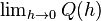$\textstyle\lim_{h\to 0} Q(h)$ exists, meaning that there is a way of choosing a value for Q(0) which makes the graph of Q a continuous function, then the function ƒ is differentiable at the point a, and its derivative at a equals Q(0).

In practice, the existence of a continuous extension of the difference quotient Q(h) to h = 0 is shown by modifying the numerator to cancel h in the denominator. This process can be long and tedious for complicated functions, and many short cuts are commonly used to simplify the process.

[edit] Example

The squaring function ƒ(x) = x² is differentiable at x = 3, and its derivative there is 6. This result is established by writing the difference quotient as follows:

${f(3+h)-f(3)\over h} = {(3+h)^2 - 9\over{h}} = {9 + 6h + h^2 - 9\over{h}} = {6h + h^2\over{h}} = 6 + h.$

Then we obtain the derivative by letting $h\to 0$ .

$(6 + h) \to 6 + 0 = 6.$

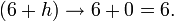
The last expression shows that the difference quotient equals 6 + h when h is not zero and is undefined when h is zero. (Remember that because of the definition of the difference quotient, the difference quotient is never defined when h is zero.) However, there is a natural way of filling in a value for the difference quotient at zero, namely 6. Hence the slope of the graph of the squaring function at the point (3, 9) is 6, and so its derivative at x = 3 is ƒ '(3) = 6.

More generally, a similar computation shows that the derivative of the squaring function at x = a is ƒ '(a) = 2a.

[edit] Continuity and differentiability

This function does not have a derivative at the marked point, as the function is not continuous there.

If y = ƒ(x) is differentiable at a, then ƒ must also be continuous at a. As an example, choose a point a and let ƒ be the step function which returns a value, say 1, for all x less than a, and returns a different value, say 10, for all x greater than or equal to a. ƒ cannot have a derivative at a. If h is negative, then a + h is on the low part of the step, so the secant line from a to a + h will be very steep, and as h tends to zero the slope tends to infinity. If h is positive, then a + h is on the high part of the step, so the secant line from a to a + h will have slope zero. Consequently the secant lines do not approach any single slope, so the limit of the difference quotient does not exist.^[4]

The absolute value function is continuous, but fails to be differentiable at x = 0 since the tangent slopes do not approach the same value from the left as they do from the right.

However, even if a function is continuous at a point, it may not be differentiable there. For example, the absolute value function y = |x| is continuous at x = 0, but it is not differentiable there. If h is positive, then the slope of the secant line from 0 to h is one, whereas if h is negative, then the slope of the secant line from 0 to h is negative one. This can be seen graphically as a "kink" in the graph at x = 0. Even a function with a smooth graph is not differentiable at a point where its tangent is vertical: For instance, the function y = ³√x is not differentiable at x = 0.

In summary: in order for a function ƒ to have a derivative it is necessary for the function ƒ to be continuous, but continuity alone is not sufficient.

Most functions which occur in practice have derivatives at all points or at almost every point. However, a result of Stefan Banach states that the set of functions which have a derivative at some point is a meager set in the space of all continuous functions.^[5] Informally, this means that differentiable functions are very atypical among continuous functions. The first known example of a function that is continuous everywhere but differentiable nowhere is the Weierstrass function.

[edit] The derivative as a function

Let ƒ be a function that has a derivative at every point a in the domain of ƒ. Because every point a has a derivative, there is a function which sends the point a to the derivative of ƒ at a. This function is written f′(x) and is called the derivative function or the derivative of ƒ. The derivative of ƒ collects all the derivatives of ƒ at all the points in the domain of ƒ.

Sometimes ƒ has a derivative at most, but not all, points of its domain. The function whose value at a equals f′(a) whenever f′(a) is defined and is undefined elsewhere is also called the derivative of ƒ. It is still a function, but its domain is strictly smaller than the domain of ƒ.

Using this idea, differentiation becomes a function of functions: The derivative is an operator whose domain is the set of all functions which have derivatives at every point of their domain and whose range is a set of functions. If we denote this operator by D, then D(ƒ) is the function f′(x). Since D(ƒ) is a function, it can be evaluated at a point a. By the definition of the derivative function, D(ƒ)(a) = f′(a).

For comparison, consider the doubling function ƒ(x) =2x; ƒ is a real-valued function of a real number, meaning that it takes numbers as inputs and has numbers as outputs:

$\begin{align} 1 &{}\mapsto 2,\\ 2 &{}\mapsto 4,\\ 3 &{}\mapsto 6. \end{align}$

The operator D, however, is not defined on individual numbers. It is only defined on functions:

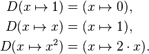
$\begin{align} D(x \mapsto 1) &= (x \mapsto 0),\\ D(x \mapsto x) &= (x \mapsto 1),\\ D(x \mapsto x^2) &= (x \mapsto 2\cdot x). \end{align}$

Because the output of D is a function, the output of D can be evaluated at a point. For instance, when D is applied to the squaring function,

$x \mapsto x^2,$

D outputs the doubling function,

$x \mapsto 2x ,$

which we named ƒ(x). This output function can then be evaluated to get ƒ(1) = 2, ƒ(2) = 4, and so on.

[edit] Higher derivatives

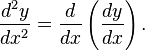
Let ƒ be a differentiable function, and let f′(x) be its derivative. The derivative of f′(x) (if it has one) is written f′′(x) and is called the second derivative of ƒ. Similarly, the derivative of a second derivative, if it exists, is written f′′′(x) and is called the third derivative of ƒ. These repeated derivatives are called higher-order derivatives.

A function ƒ need not have a derivative, for example, if it is not continuous. Similarly, even if ƒ does have a derivative, it may not have a second derivative. For example, let

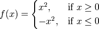$f(x) = \begin{cases} x^2, & \mbox{if }x\ge 0 \\ -x^2, & \mbox{if }x \le 0\end{cases}$ .

An elementary calculation shows that ƒ is a differentiable function whose derivative is

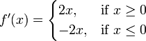$f'(x) = \begin{cases} 2x, & \mbox{if }x\ge 0 \\ -2x, & \mbox{if }x \le 0\end{cases}$ .

f′(x) is twice the absolute value function, and it does not have a derivative at zero. Similar examples show that a function can have k derivatives for any non-negative integer k but no (k + 1)-order derivative. A function that has k successive derivatives is called k times differentiable. If in addition the kth derivative is continuous, then the function is said to be of differentiability class C^k. (This is a stronger condition than having k derivatives. For an example, see differentiability class.) A function that has infinitely many derivatives is called infinitely differentiable or smooth.

On the real line, every polynomial function is infinitely differentiable. By standard differentiation rules, if a polynomial of degree n is differentiated n times, then it becomes a constant function. All of its subsequent derivatives are identically zero. In particular, they exist, so polynomials are smooth functions.

The derivatives of a function ƒ at a point x provide polynomial approximations to that function near x. For example, if ƒ is twice differentiable, then

$f(x+h) \approx f(x) + f'(x)h + \tfrac12 f''(x) h^2$

in the sense that

$\lim_{h\to 0}\frac{f(x+h) - f(x) - f'(x)h - \frac12 f''(x) h^2}{h^2}=0.$

If ƒ is infinitely differentiable, then this is the beginning of the Taylor series for ƒ.

[edit] Inflection point

Main article: Inflection point

A point where the second derivative of a function changes sign is called an inflection point.^[6] At an inflection point, the second derivative may be zero, as in the case of the inflection point x=0 of the function y=x³, or it may fail to exist, as in the case of the inflection point x=0 of the function y=x^1/3. At an inflection point, a function switches from being a convex function to being a concave function or vice versa.

[edit] Notations for differentiation

Main article: Notation for differentiation

[edit] Leibniz's notation

Main article: Leibniz's notation

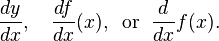
The notation for derivatives introduced by Gottfried Leibniz is one of the earliest. It is still commonly used when the equation y = ƒ(x) is viewed as a functional relationship between dependent and independent variables. Then the first derivative is denoted by

$\frac{dy}{dx},\quad\frac{d f}{dx}(x),\;\;\mathrm{or}\;\; \frac{d}{dx}f(x).$

Higher derivatives are expressed using the notation

$\frac{d^ny}{dx^n}, \quad\frac{d^n f}{dx^n}(x), \;\;\mathrm{or}\;\; \frac{d^n}{dx^n}f(x)$

for the nth derivative of y = ƒ(x) (with respect to x). These are abbreviations for multiple applications of the derivative operator. For example,

$\frac{d^2y}{dx^2} = \frac{d}{dx}\left(\frac{dy}{dx}\right).$

With Leibniz's notation, we can write the derivative of y at the point x = a in two different ways:

$\frac{dy}{dx}\left.{\!\!\frac{}{}}\right|_{x=a} = \frac{dy}{dx}(a).$

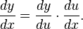
Leibniz's notation allows one to specify the variable for differentiation (in the denominator). This is especially relevant for partial differentiation. It also makes the chain rule easy to remember:^[7]

$\frac{dy}{dx} = \frac{dy}{du} \cdot \frac{du}{dx}.$

[edit] Lagrange's notation

Sometimes referred to as prime notation,^[8] one of the most common modern notations for differentiation is due to Joseph Louis Lagrange and uses the prime mark, so that the derivative of a function ƒ(x) is denoted ƒ′(x) or simply ƒ′. Similarly, the second and third derivatives are denoted

$(f')'=f''\,$ and $(f'')'=f'''\,.$

Beyond this point, some authors use Roman numerals such as

$f^{\mathrm{iv}}\,$

for the fourth derivative, whereas other authors place the number of derivatives in parentheses:

$f^{(4)}\,$

The latter notation generalizes to yield the notation ƒ ⁽ⁿ⁾ for the nth derivative of ƒ — this notation is most useful when we wish to talk about the derivative as being a function itself, as in this case the Leibniz notation can become cumbersome.

[edit] Newton's notation

Main article: Newton's notation

Newton's notation for differentiation, also called the dot notation, places a dot over the function name to represent a derivative. If y = ƒ(t), then

$\dot{y}$ and $\ddot{y}$

denote, respectively, the first and second derivatives of y with respect to t. This notation is used almost exclusively for time derivatives, meaning that the independent variable of the function represents time. It is very common in physics and in mathematical disciplines connected with physics such as differential equations. While the notation becomes unmanageable for high-order derivatives, in practice only very few derivatives are needed.

[edit] Euler's notation

Euler's notation uses a differential operator D, which is applied to a function ƒ to give the first derivative Df. The second derivative is denoted D²ƒ, and the nth derivative is denoted Dⁿƒ.

If y = ƒ(x) is a dependent variable, then often the subscript x is attached to the D to clarify the independent variable x. Euler's notation is then written

$D_x y\,$ or $D_x f(x)\,$ ,

although this subscript is often omitted when the variable x is understood, for instance when this is the only variable present in the expression.

Euler's notation is useful for stating and solving linear differential equations.

[edit] Computing the derivative

The derivative of a function can, in principle, be computed from the definition by considering the difference quotient, and computing its limit. For some examples, see Derivative (examples). In practice, once the derivatives of a few simple functions are known, the derivatives of other functions are more easily computed using rules for obtaining derivatives of more complicated functions from simpler ones.

[edit] Derivatives of elementary functions

Main article: Table of derivatives

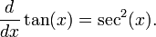
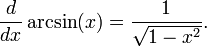
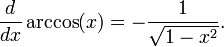
Most derivative computations eventually require taking the derivative of some common functions. The following incomplete list gives some of the most frequently used functions of a single real variable and their derivatives. For a complete list, see Table of derivatives.

Derivatives of powers: if

$f(x) = x^r\,$ ,

where r is any real number, then

$f'(x) = rx^{r-1}\,$ ,

wherever this function is defined. For example, if r = 1/2, then

$f'(x) = \frac{1}{2}x^{-\tfrac12}\,$ .

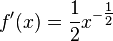and the function is defined only for non-negative x. When r = 0, this rule recovers the constant rule.

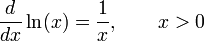
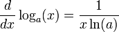
Exponential and logarithmic functions:

$\frac{d}{dx}e^x = e^x$

$\frac{d}{dx}a^x = \ln(a)a^x$

$\frac{d}{dx}\ln(x) = \frac{1}{x},\qquad x > 0$

$\frac{d}{dx}\log_a(x) = \frac{1}{x\ln(a)}$

Trigonometric functions:

$\frac{d}{dx}\sin(x) = \cos(x).$

$\frac{d}{dx}\cos(x)= -\sin(x).$

$\frac{d}{dx}\tan(x)= \sec^2(x).$

Inverse trigonometric functions:

$\frac{d}{dx}\arcsin(x) = \frac{1}{\sqrt{1-x^2}}.$

$\frac{d}{dx}\arccos(x)= -\frac{1}{\sqrt{1-x^2}}.$

$\frac{d}{dx}\arctan(x)= \frac{1}{{1+x^2}}.$

[edit] Rules for finding the derivative

Main article: Differentiation rules

In many cases, complicated limit calculations by direct application of Newton's difference quotient can be avoided using differentiation rules. Some of the most basic rules are the following.

Constant rule: if ƒ(x) is constant, then

$f' = 0 \,$

Sum rule:

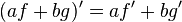$(af + bg)' = af' + bg' \,$ for all functions ƒ and g and all real numbers a and b.

Product rule:

$(fg)' = f 'g + fg' \,$ for all functions ƒ and g.

Quotient rule:

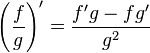$\left(\frac{f}{g} \right)' = \frac{f'g - fg'}{g^2}$ for all functions ƒ and g where g ≠ 0.

Chain rule: If $f (x) = h (g (x))$ , then

$f'(x) = h'(g(x)) \cdot g'(x) \,$ .

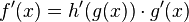[edit] Example computation

The derivative of

$f(x) = x^4 + \sin (x^2) - \ln(x) e^x + 7\,$

is

$\begin{align} f'(x) &= 4 x^{(4-1)}+ \frac{d\left(x^2\right)}{dx}\cos (x^2) - \frac{d\left(\ln {x}\right)}{dx} e^x - \ln{x} \frac{d\left(e^x\right)}{dx} + 0 \\ &= 4x^3 + 2x\cos (x^2) - \frac{1}{x} e^x - \ln(x) e^x. \end{align}$

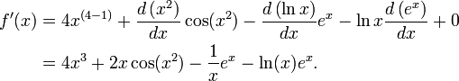
Here the second term was computed using the chain rule and third using the product rule. The known derivatives of the elementary functions x², x⁴, sin(x), ln(x) and exp(x) = e^x, as well as the constant 7, were also used.

[edit] Derivatives in higher dimensions

See also: Vector calculus and Multivariable calculus

[edit] Derivatives of vector valued functions

A vector-valued function y(t) of a real variable is a function which sends real numbers to vectors in some vector space Rⁿ. A vector-valued function can be split up into its coordinate functions y₁(t), y₂(t), …, y_n(t), meaning that y(t) = (y₁(t), ..., y_n(t)). This includes, for example, parametric curves in R² or R³. The coordinate functions are real valued functions, so the above definition of derivative applies to them. The derivative of y(t) is defined to be the vector, called the tangent vector, whose coordinates are the derivatives of the coordinate functions. That is,

$\mathbf{y}'(t) = (y'_1(t), \ldots, y'_n(t)).$

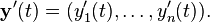
Equivalently,

$\mathbf{y}'(t)=\lim_{h\to 0}\frac{\mathbf{y}(t+h) - \mathbf{y}(t)}{h},$

if the limit exists. The subtraction in the numerator is subtraction of vectors, not scalars. If the derivative of y exists for every value of t, then y′ is another vector valued function.

If e₁, …, e_n is the standard basis for Rⁿ, then y(t) can also be written as y₁(t)e₁ + … + y_n(t)e_n. If we assume that the derivative of a vector-valued function retains the linearity property, then the derivative of y(t) must be

$y'_1(t)\mathbf{e}_1 + \cdots + y'_n(t)\mathbf{e}_n$

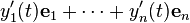
because each of the basis vectors is a constant.

This generalization is useful, for example, if y(t) is the position vector of a particle at time t; then the derivative y′(t) is the velocity vector of the particle at time t.

[edit] Partial derivatives

Main article: Partial derivative

Suppose that ƒ is a function that depends on more than one variable. For instance,

$f(x,y) = x^2 + xy + y^2.\,$

ƒ can be reinterpreted as a family of functions of one variable indexed by the other variables:

$f(x,y) = f_x(y) = x^2 + xy + y^2.\,$

In other words, every value of x chooses a function, denoted f_x, which is a function of one real number.^[9] That is,

$x \mapsto f_x,\,$

$f_x(y) = x^2 + xy + y^2.\,$

Once a value of x is chosen, say a, then f(x,y) determines a function f_a which sends y to a² + ay + y²:

$f_a(y) = a^2 + ay + y^2.\,$

In this expression, a is a constant, not a variable, so f_a is a function of only one real variable. Consequently the definition of the derivative for a function of one variable applies:

$f_a'(y) = a + 2y.\,$

The above procedure can be performed for any choice of a. Assembling the derivatives together into a function gives a function which describes the variation of ƒ in the y direction:

$\frac{\part f}{\part y}(x,y) = x + 2y.$

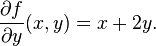
This is the partial derivative of ƒ with respect to y. Here ∂ is a rounded d called the partial derivative symbol. To distinguish it from the letter d, ∂ is sometimes pronounced "der", "del", or "partial" instead of "dee".

In general, the partial derivative of a function ƒ(x₁, …, x_n) in the direction x_i at the point (a₁ …, a_n) is defined to be:

$\frac{\part f}{\part x_i}(a_1,\ldots,a_n) = \lim_{h \to 0}\frac{f(a_1,\ldots,a_i+h,\ldots,a_n) - f(a_1,\ldots,a_n)}{h}.$

In the above difference quotient, all the variables except x_i are held fixed. That choice of fixed values determines a function of one variable

$f_{a_1,\ldots,a_{i-1},a_{i+1},\ldots,a_n}(x_i) = f(a_1,\ldots,a_{i-1},x_i,a_{i+1},\ldots,a_n)$

and, by definition,

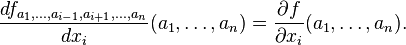
$\frac{df_{a_1,\ldots,a_{i-1},a_{i+1},\ldots,a_n}}{dx_i}(a_1,\ldots,a_n) = \frac{\part f}{\part x_i}(a_1,\ldots,a_n).$

In other words, the different choices of a index a family of one-variable functions just as in the example above. This expression also shows that the computation of partial derivatives reduces to the computation of one-variable derivatives.

An important example of a function of several variables is the case of a scalar-valued function ƒ(x₁,...x_n) on a domain in Euclidean space Rⁿ (e.g., on R² or R³). In this case ƒ has a partial derivative ∂ƒ/∂x_j with respect to each variable x_j. At the point a, these partial derivatives define the vector

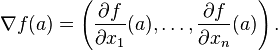
$\nabla f(a) = \left(\frac{\partial f}{\partial x_1}(a), \ldots, \frac{\partial f}{\partial x_n}(a)\right).$

This vector is called the gradient of ƒ at a. If ƒ is differentiable at every point in some domain, then the gradient is a vector-valued function ∇ƒ which takes the point a to the vector ∇f(a). Consequently the gradient determines a vector field.

[edit] Directional derivatives

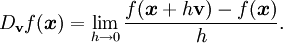
Main article: Directional derivative

If ƒ is a real-valued function on Rⁿ, then the partial derivatives of ƒ measure its variation in the direction of the coordinate axes. For example, if ƒ is a function of x and y, then its partial derivatives measure the variation in ƒ in the x direction and the y direction. They do not, however, directly measure the variation of ƒ in any other direction, such as along the diagonal line y = x. These are measured using directional derivatives. Choose a vector

$\mathbf{v} = (v_1,\ldots,v_n).$

The directional derivative of ƒ in the direction of v at the point x is the limit

$D_{\mathbf{v}}{f}(\boldsymbol{x}) = \lim_{h \rightarrow 0}{\frac{f(\boldsymbol{x} + h\mathbf{v}) - f(\boldsymbol{x})}{h}}.$

Let λ be a scalar. The substitution of h/λ for h changes the λv direction's difference quotient into λ times the v direction's difference quotient. Consequently, the directional derivative in the λv direction is λ times the directional derivative in the v direction. Because of this, directional derivatives are often considered only for unit vectors v.

If all the partial derivatives of ƒ exist and are continuous at x, then they determine the directional derivative of ƒ in the direction v by the formula:

$D_{\mathbf{v}}{f}(\boldsymbol{x}) = \sum_{j=1}^n v_j \frac{\partial f}{\partial x_j}.$

This is a consequence of the definition of the total derivative. It follows that the directional derivative is linear in v.

The same definition also works when ƒ is a function with values in R^m. We just use the above definition in each component of the vectors. In this case, the directional derivative is a vector in R^m.

[edit] The total derivative, the total differential and the Jacobian

Main article: Total derivative

Let ƒ be a function from a domain in R to R. The derivative of ƒ at a point a in its domain is the best linear approximation to ƒ at that point. As above, this is a number. Geometrically, if v is a unit vector starting at a, then f′ (a) , the best linear approximation to ƒ at a, should be the length of the vector found by moving v to the target space using ƒ. (This vector is called the pushforward of v by ƒ and is usually written $f * v$ .) In other words, if v is measured in terms of distances on the target, then, because v can only be measured through ƒ, v no longer appears to be a unit vector because ƒ does not preserve unit vectors. Instead v appears to have length f′ (a). If m is greater than one, then by writing ƒ using coordinate functions, the length of v in each of the coordinate directions can be measured separately.

Suppose now that ƒ is a function from a domain in Rⁿ to R^m and that a is a point in the domain of ƒ. The derivative of ƒ at a should still be the best linear approximation to ƒ at a. In other words, if v is a vector on Rⁿ, then f′ (a) should be the linear transformation that best approximates ƒ at a. The linear transformation should contain all the information about how ƒ transforms vectors at a to vectors at f(a), and in symbols, this means it should be the linear transformation f′ (a) such that

$\lim_{\|\mathbf{h}\|\rightarrow 0} \frac{\|f(\mathbf{a}+\mathbf{h}) - f(\mathbf{a}) - f'(\mathbf{a})(\mathbf{h})\|}{\|\mathbf{h}\|} = 0.$

Here h is a vector in Rⁿ, so the norm in the denominator is the standard length on Rⁿ. However, f′ (a)h is a vector in R^m, and the norm in the numerator is the standard length on R^m. The linear transformation f′ (a), if it exists, is called the total derivative of ƒ at a or the (total) differential of ƒ at a.

If the total derivative exists at a, then all the partial derivatives of ƒ exist at a. If we write ƒ using coordinate functions, so that ƒ = (ƒ₁, ƒ₂, ..., ƒ_m), then the total derivative can be expressed as a matrix called the Jacobian matrix of ƒ at a:

$f'(\mathbf{a}) = \text{Jac}_{\mathbf{a}} = \left(\frac{\partial f_i}{\partial x_j}\right)_{ij}.$

The existence of the total derivative f′ (a) is strictly stronger than the existence of all the partial derivatives, but if the partial derivatives exist and satisfy mild smoothness conditions, then the total derivative exists and is given by the Jacobian.

The definition of the total derivative subsumes the definition of the derivative in one variable. In this case, the total derivative exists if and only if the usual derivative exists. The Jacobian matrix reduces to a 1×1 matrix whose only entry is the derivative f′ (x). This 1×1 matrix satisfies the property that ƒ(a + h) − ƒ(a) − f′(a)h is approximately zero, in other words that

$f(a+h) \approx f(a) + f'(a)h.$

Up to changing variables, this is the statement that the function $x \mapsto f(a) + f'(a)(x-a)$ is the best linear approximation to ƒ at a.

The total derivative of a function does not give another function in the same way as the one-variable case. This is because the total derivative of a multivariable function has to record much more information than the derivative of a single-variable function. Instead, the total derivative gives a function from the tangent bundle of the source to the tangent bundle of the target.

[edit] Generalizations

Main article: Derivative (generalizations)

The concept of a derivative can be extended to many other settings. The common thread is that the derivative of a function at a point serves as a linear approximation of the function at that point.

An important generalization of the derivative concerns complex functions of complex variables, such as functions from (a domain in) the complex numbers C to C. The notion of the derivative of such a function is obtained by replacing real variables with complex variables in the definition. However, this innocent definition hides some very deep properties. If C is identified with R² by writing a complex number z as x + i y, then a differentiable function from C to C is certainly differentiable as a function from R² to R² (in the sense that its partial derivatives all exist), but the converse is not true in general: the complex derivative only exists if the real derivative is complex linear and this imposes relations between the partial derivatives called the Cauchy Riemann equations — see holomorphic functions.

Another generalization concerns functions between differentiable or smooth manifolds. Intuitively speaking such a manifold M is a space which can be approximated near each point x by a vector space called its tangent space: the prototypical example is a smooth surface in R³. The derivative (or differential) of a (differentiable) map ƒ: M → N between manifolds, at a point x in M, is then a linear map from the tangent space of M at x to the tangent space of N at ƒ(x). The derivative function becomes a map between the tangent bundles of M and N. This definition is fundamental in differential geometry and has many uses — see pushforward (differential) and pullback (differential geometry).

Differentiation can also be defined for maps between infinite dimensional vector spaces such as Banach spaces and Fréchet spaces. There is a generalization both of the directional derivative, called the Gâteaux derivative, and of the differential, called the Fréchet derivative.

One deficiency of the classical derivative is that not very many functions are differentiable. Nevertheless, there is a way of extending the notion of the derivative so that all continuous functions and many other functions can be differentiated using a concept known as the weak derivative. The idea is to embed the continuous functions in a larger space called the space of distributions and only require that a function is differentiable "on average".

The properties of the derivative have inspired the introduction and study of many similar objects in algebra and topology — see, for example, differential algebra.

Also see arithmetic derivative.

[edit] See also

Mathematics portal

[edit] Notes

^ Differential calculus, as discussed in this article, is a very well-established mathematical discipline for which there are many sources. Almost all of the material in this article can be found in Apostol 1967, Apostol 1969, and Spivak 1994.
^ Spivak 1994, chapter 10.
^ See Differential (infinitesimal) for an overview. Further approaches include the Radon-Nikodym theorem, and the universal derivation (see Kähler differential).
^ Despite this, it is still possible to take the derivative in the sense of distributions. The result is nine times the Dirac measure centered at a.
^ Banach, S. (1931). "Uber die Baire'sche Kategorie gewisser Funktionenmengen". Studia. Math. (3): 174–179. . Cited by Hewitt, E and Stromberg, K (1963). Real and abstract analysis. Springer-Verlag. Theorem 17.8.
^ Apostol 1967, §4.18
^ In the formulation of calculus in terms of limits, the du symbol has been assigned various meanings by various authors. Some authors do not assign a meaning to du by itself, but only as part of the symbol du/dx. Others define "dx" as an independent variable, and define du by du = dx•ƒ′ (x). In non-standard analysis du is defined as an infinitesimal. It is also interpreted as the exterior derivative du of a function u. See differential (infinitesimal) for further information.
^ [1]
^ This can also be expressed as the adjointness between the product space and function space constructions.

[edit] References

[edit] Print

Anton, Howard; Bivens, Irl; Davis, Stephen (February 2, 2005), Calculus: Early Transcendentals Single and Multivariable (8th ed.), New York: Wiley, ISBN 978-0471472445
Apostol, Tom M. (June 1967), Calculus, Vol. 1: One-Variable Calculus with an Introduction to Linear Algebra, 1 (2nd ed.), Wiley, ISBN 978-0471000051
Apostol, Tom M. (June 1969), Calculus, Vol. 2: Multi-Variable Calculus and Linear Algebra with Applications, 1 (2nd ed.), Wiley, ISBN 978-0471000075
Eves, Howard (January 2, 1990), An Introduction to the History of Mathematics (6th ed.), Brooks Cole, ISBN 978-0030295584
Larson, Ron; Hostetler, Robert P.; Edwards, Bruce H. (February 28, 2006), Calculus: Early Transcendental Functions (4th ed.), Houghton Mifflin Company, ISBN 978-0618606245
Spivak, Michael (September 1994), Calculus (3rd ed.), Publish or Perish, ISBN 978-0914098898
Stewart, James (December 24, 2002), Calculus (5th ed.), Brooks Cole, ISBN 978-0534393397
Thompson, Silvanus P. (September 8, 1998), Calculus Made Easy (Revised, Updated, Expanded ed.), New York: St. Martin's Press, ISBN 978-0312185480

[edit] Online books

Crowell, Benjamin (2003), Calculus, http://www.lightandmatter.com/calc/
Garrett, Paul (2004), Notes on First-Year Calculus, http://www.math.umn.edu/~garrett/calculus/
Hussain, Faraz (2006), Understanding Calculus, http://www.understandingcalculus.com/
Keisler, H. Jerome (2000), Elementary Calculus: An Approach Using Infinitesimals, http://www.math.wisc.edu/~keisler/calc.html
Mauch, Sean (2004), Unabridged Version of Sean's Applied Math Book, http://www.its.caltech.edu/~sean/book/unabridged.html
Sloughter, Dan (2000), Difference Equations to Differential Equations, http://synechism.org/drupal/de2de/
Strang, Gilbert (1991), Calculus, http://ocw.mit.edu/ans7870/resources/Strang/strangtext.htm
Stroyan, Keith D. (1997), A Brief Introduction to Infinitesimal Calculus, http://www.math.uiowa.edu/~stroyan/InfsmlCalculus/InfsmlCalc.htm
Wikibooks, Calculus, http://en.wikibooks.org/wiki/Calculus

[edit] External links

WIMS Function Calculator makes online calculation of derivatives; this software also enables interactive exercises.
Mathematical Assistant on Web online calculation of derivatives, including explanation of steps in the solution.
Practice finding derivatives of randomly generated functions

[0] Differential calculus, as discussed in this article, is a very well-established mathematical discipline for which there are many sources. Almost all of the material in this article can be found in Apostol 1967, Apostol 1969, and Spivak 1994.

[1] Spivak 1994, chapter 10.

[2] See Differential (infinitesimal) for an overview. Further approaches include the Radon-Nikodym theorem, and the universal derivation (see Kähler differential).

[3] Despite this, it is still possible to take the derivative in the sense of distributions. The result is nine times the Dirac measure centered at a.

[4] Banach, S. (1931). "Uber die Baire'sche Kategorie gewisser Funktionenmengen". Studia. Math. (3): 174–179. . Cited by Hewitt, E and Stromberg, K (1963). Real and abstract analysis. Springer-Verlag. Theorem 17.8.

[5] Apostol 1967, §4.18

[6] In the formulation of calculus in terms of limits, the du symbol has been assigned various meanings by various authors. Some authors do not assign a meaning to du by itself, but only as part of the symbol du/dx. Others define "dx" as an independent variable, and define du by du = dx•ƒ′ (x). In non-standard analysis du is defined as an infinitesimal. It is also interpreted as the exterior derivative du of a function u. See differential (infinitesimal) for further information.

[7] [1]

[8] This can also be expressed as the adjointness between the product space and function space constructions.

[1]

[2]

[3]

[4]

[5]

[6]

[7]

[8]

[9]