Linear regression

From Wikipedia, the free encyclopedia

In statistics, linear regression is used for two things;

to construct a simple formula that will predict what value will occur for a quantity of interest when other related variables take given values.
to allow a test to be made of whether a given variable does have an effect on a quantity of interest in situations where there may be many related variables.

In both cases, several sets of outcomes are available for the quantity of interest together with the related variables.

Linear regression is a form of regression analysis in which the relationship between one or more independent variables and another variable, called the dependent variable, is modelled by a least squares function, called a linear regression equation. This function is a linear combination of one or more model parameters, called regression coefficients. A linear regression equation with one independent variable represents a straight line when the predicted value (i.e. the dependant variable from the regression equation) is plotted against the independent variable: this is called a simple linear regression. However, note that "linear" does not refer to this straight line, but rather to the way in which the regression coefficients occur in the regression equation. The results are subject to statistical analysis.

Example of linear regression with one independent variable.

[edit] Introduction

[edit] Theoretical model

A linear regression model assumes, given a random sample $(Y_i, X_{i1}, \ldots, X_{ip}), \, i = 1, \ldots, n$ , a possibly imperfect relationship between $Y i$ , the regressand, and regressors $X_{i1}, \ldots, X_{ip}$ . A disturbance term $\varepsilon_i$ , which is a random variable too, is added to this assumed relationship to capture the influence of everything else on $Y i$ other than $X_{i1}, \ldots, X_{ip}$ . Hence, the multiple linear regression model takes the following form:

$Y_i = \beta_0 + \beta_1 X_{i1} + \beta_2 X_{i2} + \cdots + \beta_p X_{ip} + \varepsilon_i, \qquad i = 1, \ldots, n$

Note that the regressors are also called independent variables, exogenous variables, covariates, input variables or predictor variables. Similarly, regressands are also called dependent variables, response variables, measured variables, or predicted variables.

Models which do not conform to this specification may be treated by nonlinear regression. A linear regression model need not be a linear function of the independent variable: linear in this context means that the conditional mean of $Y i$ is linear in the parameters $β$ . For example, the model $Y_i = \beta_1 X_i + \beta_2 X_i^2 + \varepsilon_i$ is linear in the parameters $β 1$ and $β 2$ , but it is not linear in $X_i^2$ , a nonlinear function of $X i$ . An illustration of this model is shown in the example, below.

[edit] Data and estimation

It is important to distinguish the model formulated in terms of random variables and the observed values of these random variables. Typically, the observed values, or data, denoted by lower case letters, consist of n values $(y_i, x_{i1}, \ldots, x_{ip}), \, i = 1, \ldots, n$ .

In general there are $p + 1$ parameters to be determined, $\beta_0, \ldots, \beta_p$ . In order to estimate the parameters it is often useful to use the matrix notation

$Y = X \beta + \varepsilon \,$

where Y is a column vector that includes the observed values of $Y_1, \ldots, Y_n$ , $\varepsilon$ includes the unobserved stochastic components $\varepsilon_1, \ldots, \varepsilon_n$ and the matrix $X$ the observed values of the regressors

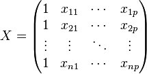
$X = \begin{pmatrix} 1 & x_{11} & \cdots & x_{1p} \\ 1 & x_{21} & \cdots & x_{2p}\\ \vdots & \vdots & \ddots & \vdots \\ 1 & x_{n1} & \cdots & x_{np} \end{pmatrix}$

X includes, typically, a constant column, that is, a column which does not vary across observations, which is used to represent the intercept term $β 0$ .

If there is any linear dependence among the columns of X, then the vector of parameters $β$ cannot be estimated by least squares unless $β$ is constrained, as, for example, by requiring the sum of some of its components to be 0. However, some linear combinations of the components of $β$ may still be uniquely estimable in such cases. For example, the model $Y_i = \beta_1 X_i + \beta_2 2 X_i + \varepsilon_i$ cannot be solved for $β 1$ and $β 2$ independently as the matrix of observations has the reduced rank 2. In this case the model can be rewritten as $Y_i = (\beta_1 + 2\beta_2)X_i + \varepsilon_i$ and can be solved to give a value for the composite entity $β 1 + 2β 2$ .

Note that to only perform a least squares estimation of $\beta_0, \beta_1, \ldots, \beta_p$ it is not necessary to consider the sample as random variables. It may even be conceptually simpler to consider the sample as fixed, observed values, as we have done thus far. However in the context of hypothesis testing and confidence intervals, it will be necessary to interpret the sample as random variables $(Y_i, X_{i1}, \ldots, X_{ip}), \, i = 1, \ldots, n$ that will produce estimators which are themselves random variables. Then it will be possible to study the distribution of the estimators and draw inferences.

[edit] Classical assumptions

Classical assumptions for linear regression include the assumptions that the sample is selected at random from the population of interest, that the dependent variable is continuous on the real line, and that the error terms follow identical and independent normal distributions, that is, that the errors are i.i.d. and Gaussian. Note that these assumptions imply that the error term does not statistically depend on the values of the independent variables, that is, that $\varepsilon_i$ is statistically independent of the predictor variables. This article adopts these assumptions unless otherwise stated. Note that all of these assumptions may be relaxed, depending on the nature of the true probabilistic model of the problem at hand. The issue of choosing which assumptions to relax, which functional form to adopt, and other choices related to the underlying probabilistic model are known as specification searches. In particular note that the assumption that the error terms are normally distributed is of no consequence unless the sample is very small because central limit theorems imply that, so long as the error terms have finite variance and are not too strongly correlated, the parameter estimates will be approximately normally distributed even when the underlying errors are not.

Under these assumptions, an equivalent formulation of simple linear regression that explicitly shows the linear regression as a model of conditional expectation can be given as

$\mbox{E}(Y_i \mid X_i = x_i) = \alpha + \beta x_i \,$

The conditional expected value of Y_i given X_i is an affine function of X_i. Note that this expression follows from the assumption that the mean of $\varepsilon_i$ is zero conditional on X_i.

[edit] Least-squares analysis

[edit] Least squares estimates

The first objective of regression analysis is to best-fit the data by estimating the parameters of the model. Of the different criteria that can be used to define what constitutes a best fit, the least squares criterion is a very powerful one. This estimate (or estimator, if we are in the context of a random sample), is given by

$\hat\beta = (X^T X)^{-1}X^T y \,$

For a full derivation see Linear least squares.

[edit] Regression inference

The estimates can be used to test various hypotheses.

Denote by $σ 2$ the variance of the error term $\varepsilon$ (recall we assume that $\varepsilon_i \sim N(0,\sigma^2)\,$ for every $i=1,\ldots,n$ ). An unbiased estimate of $σ 2$ is given by

$\hat \sigma^2 = \frac {S} {n-p} ,$

where $S := \sum_{i=1}^n \hat{\varepsilon}_i^2$ is the sum of square residuals. The relation between the estimate and the true value is:

$\hat\sigma^2 \cdot \frac{n-p}{\sigma^2} \sim \chi_{n-p}^2$

where $\chi_{n-p}^2$ has Chi-square distribution with n − p degrees of freedom.

The solution to the normal equations can be written as ^[1]

$\hat\boldsymbol\beta=(\mathbf{X^TX)^{-1}X^Ty}.$

This shows that the parameter estimators are linear combinations of the dependent variable. It follows that, if the observational errors are normally distributed, the parameter estimators will follow a joint normal distribution. Under the assumptions here, the estimated parameter vector is exactly distributed,

$\hat\beta \sim N ( \beta, \sigma^2 (X^TX)^{-1} )$

where N denotes the multivariate normal distribution.

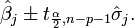
The standard error of a parameter estimator is given by

$\hat\sigma_j=\sqrt{ \frac{S}{n-p-1}\left[\mathbf{(X^TX)}^{-1}\right]_{jj}}.$

The 100(1 − α)% confidence interval for the parameter, $β j$ , is computed as follows:

$\hat \beta_j \pm t_{\frac{\alpha }{2},n - p - 1} \hat \sigma_j.$

The residuals can be expressed as

$\mathbf{\hat r = y-X \hat\boldsymbol\beta= y-X(X^TX)^{-1}X^Ty}.\,$

The matrix $\mathbf{X(X^TX)^{-1}X^T}$ is known as the hat matrix and has the useful property that it is idempotent. Using this property it can be shown that, if the errors are normally distributed, the residuals will follow a normal distribution with covariance matrix 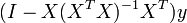$(I - X(X^TX)^{-1}X^T)y\,$ . Studentized residuals are useful in testing for outliers.

The hat matrix is the matrix of the orthogonal projection onto the column space of the matrix X.

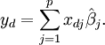
Given a value of the independent variable, x_d, the predicted response is calculated as

$y_d=\sum_{j=1}^{p}x_{dj}\hat\beta_j.$

Writing the elements $x_{dj},\ j=1,p$ as $\mathbf z$ , the 100(1 − α)% mean response confidence interval for the prediction is given, using error propagation theory, by:

$\mathbf{z^T\hat\boldsymbol\beta} \pm t_{ \frac{\alpha }{2} ,n-p} \hat \sigma \sqrt {\mathbf{ z^T(X^T X)^{- 1}z }}.$

The 100(1 − α)% predicted response confidence intervals for the data are given by:

$\mathbf z^T \hat\boldsymbol\beta \pm t_{\frac{\alpha }{2},n-p-1} \hat \sigma \sqrt {1 + \mathbf{z^T(X^TX)^{-1}z}}.$

[edit] Univariate linear case

We consider here the case of the simplest regression model, $Y = \alpha + \beta X + \varepsilon$ . In order to estimate $α$ and $β$ , we have a sample $(y_i, x_i), \, i = 1, \ldots, n$ of observations which are, here, not seen as random variables and denoted by lower case letters. As stated in the introduction, however, we might want to interpret the sample in terms of random variables in some other contexts than least squares estimation.

The idea of least squares estimation is to minimize the following unknown quantity, the sum of squared errors:

$\sum_{i = 1}^n \varepsilon_i^2 = \sum_{i = 1}^n (y_i - \alpha - \beta x_i)^2$

Taking the derivative of the preceding expression with respect to $α$ and $β$ yields the normal equations:

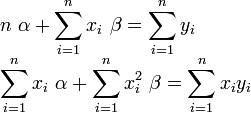
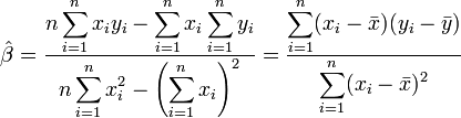
$\begin{array}{lcl} n\ \alpha + \displaystyle\sum_{i = 1}^n x_i\ \beta = \displaystyle\sum_{i = 1}^n y_i \\ \displaystyle\sum_{i = 1}^n x_i\ \alpha + \displaystyle\sum_{i = 1}^n x_i^2\ \beta = \displaystyle\sum_{i = 1}^n x_i y_i \end{array}$

This is a linear system of equations which can be solved using Cramer's rule:

$\hat\beta = \frac {n \displaystyle\sum_{i = 1}^n x_i y_i - \displaystyle\sum_{i = 1}^n x_i \displaystyle\sum_{i = 1}^n y_i} {n \displaystyle\sum_{i = 1}^n x_i^2 - \left(\displaystyle\sum_{i = 1}^n x_i\right)^2} =\frac{\displaystyle\sum_{i = 1}^n(x_i-\bar{x})(y_i-\bar{y})}{\displaystyle\sum_{i = 1}^n(x_i-\bar{x})^2} \,$

$\hat\alpha = \frac {\displaystyle\sum_{i = 1}^n x_i^2 \displaystyle\sum_{i = 1}^n y_i - \displaystyle\sum_{i = 1}^n x_i \displaystyle\sum_{i = 1}^n x_iy_i} {n \displaystyle\sum_{i = 1}^n x_i^2 - \left(\displaystyle\sum_{i = 1}^n x_i\right)^2}= \bar y-\bar x \hat\beta$

$S = \sum_{i = 1}^n (y_i - \hat{y}_i)^2 = \sum_{i = 1}^n y_i^2 - \frac {n \left(\displaystyle\sum_{i = 1}^n x_i y_i \right)^2 + \left(\displaystyle\sum_{i = 1}^n y_i \right)^2 \displaystyle\sum_{i = 1}^n x_i^2 - 2 \displaystyle\sum_{i = 1}^n x_i \displaystyle\sum_{i = 1}^n y_i \displaystyle\sum_{i = 1}^n x_i y_i } {n \displaystyle\sum_{i = 1}^n x_i^2 - \left(\displaystyle\sum_{i = 1}^n x_i\right)^2}$

$\hat \sigma^2 = \frac {S} {n-2}.$

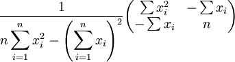
The covariance matrix is

$\frac{1}{n \displaystyle\sum_{i = 1}^n x_i^2 - \left(\displaystyle\sum_{i = 1}^n x_i\right)^2}\begin{pmatrix} \sum x_i^2 & -\sum x_i \\ -\sum x_i & n \end{pmatrix}$

The mean response confidence interval is given by

$y_d = (\alpha+\hat\beta x_d) \pm t_{ \frac{\alpha }{2} ,n-2} \hat \sigma \sqrt {\frac{1}{n} + \frac{(x_d - \bar{x})^2}{\sum (x_i - \bar{x})^2}}$

The predicted response confidence interval is given by

$y_d = (\alpha+\hat\beta x_d) \pm t_{ \frac{\alpha }{2} ,n-2} \hat \sigma \sqrt {1+\frac{1}{n} + \frac{(x_d - \bar{x})^2}{\sum (x_i - \bar{x})^2}}$

The term $t_{ \frac{\alpha }{2} ,n-2}$ is a reference to the Student's t-distribution. $\hat \sigma$ is standard error.

[edit] Analysis of variance

In analysis of variance (ANOVA), the total sum of squares is split into two or more components.

The "total (corrected) sum of squares" is

$\text{SST} = \sum_{i=1}^n (y_i - \bar y)^2,$

where

$\bar y = \frac{1}{n} \sum_i y_i$

("corrected" means $\scriptstyle\bar y\,$ has been subtracted from each y-value). Equivalently

$\text{SST} = \sum_{i=1}^n y_i^2 - \frac{1}{n}\left(\sum_i y_i\right)^2$

The total sum of squares is partitioned as the sum of the "regression sum of squares" SSReg (or RSS, also called the "explained sum of squares") and the "error sum of squares" SSE, which is the sum of squares of residuals.

The regression sum of squares is

$\text{SSReg} = \sum \left( \hat y_i - \bar y \right)^2 = \hat\boldsymbol\beta^T \mathbf{X}^T \mathbf y - \frac{1}{n}\left( \mathbf {y^T u u^T y} \right),$

where u is an n-by-1 vector in which each element is 1. Note that

$\mathbf{y^T u} = \mathbf{u^T y} = \sum_i y_i,$

and

$\frac{1}{n} \mathbf{y^T u u^T y} = \frac{1}{n}\left(\sum_i y_i\right)^2.\,$

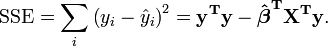
The error (or "unexplained") sum of squares SSE, which is the sum of square of residuals, is given by

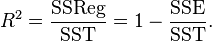
$\text{SSE} = \sum_i {\left( {y_i - \hat y_i} \right)^2 } = \mathbf{ y^T y - \hat\boldsymbol\beta^T X^T y}.$

The total sum of squares SST is

$\text{SST} = \sum_i \left( y_i-\bar y \right)^2 = \mathbf{ y^T y}-\frac{1}{n}\left( \mathbf{y^Tuu^Ty}\right)=\text{SSReg}+ \text{SSE}.$

Pearson's coefficient of regression, R² is then given as

$R^2 = \frac{\text{SSReg}}{{\text{SST}}} = 1 - \frac{\text{SSE}}{\text{SST}}.$

If the errors are independent and normally distributed with expected value 0 and they all have the same variance, then under the null hypothesis that all of the elements in β = 0 except the constant, the statistic

$\frac{ R^2 / ( m-1 ) }{ ( 1 - R^2 )/(n-m)}$

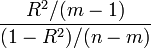
follows an F-distribution with (m-1) and (n-m) degrees of freedom. If that statistic is too large, then one rejects the null hypothesis. How large is too large depends on the level of the test, which is the tolerated probability of type I error; see [statistical significance]].

[edit] Example

To illustrate the various goals of regression, we give an example. The following data set gives the average heights and weights for American women aged 30-39 (source: The World Almanac and Book of Facts, 1975).

Height (m)	1.47	1.5	1.52	1.55	1.57	1.60	1.63	1.65	1.68	1.7	1.73	1.75	1.78	1.8	1.83
Weight (kg)	52.21	53.12	54.48	55.84	57.2	58.57	59.93	61.29	63.11	64.47	66.28	68.1	69.92	72.19	74.46

A plot of weight against height (see below) shows that it cannot be modeled by a straight line, so a regression is performed by modeling the data by a parabola.

$Y_i = \beta_0 + \beta_1 X_i + \beta_2 X^2_i +\varepsilon_i \!$

where the dependent variable $Y i$ is weight and the independent variable $X i$ is height.

Place the observations $x_i, \ x_i^2, \, i = 1, \ldots, n$ , in the matrix X.

$\mathbf{X} = \begin{pmatrix} 1&1.47&2.16\\ 1&1.50&2.25\\ 1&1.52&2.31\\ 1&1.55&2.40\\ 1&1.57&2.46\\ 1&1.60&2.56\\ 1&1.63&2.66\\ 1&1.65&2.72\\ 1&1.68&2.82\\ 1&1.70&2.89\\ 1&1.73&2.99\\ 1&1.75&3.06\\ 1&1.78&3.17\\ 1&1.80&3.24\\ 1&1.83&3.35\\ \end{pmatrix}$

The values of the parameters are found by solving the normal equations

$\mathbf{(X^TX)\boldsymbol\hat\beta=X^Ty}$

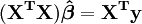
Element ij of the normal equation matrix, $\mathbf{X^TX}$ is formed by summing the products of column i and column j of X.

$x_{ij} = \sum_{k = 1}^{15} x_{ki} x_{kj}$

Element i of the right-hand side vector $\mathbf{X^Ty}$ is formed by summing the products of column i of X with the column of dependent variable values.

$\left(\mathbf{X^Ty}\right)_i= \sum_{k = 1}^{15} x_{ki} y_k$

Thus, the normal equations are

$\begin{pmatrix} 15&24.76&41.05\\ 24.76&41.05&68.37\\ 41.05&68.37&114.35\\ \end{pmatrix} \begin{pmatrix} \hat\beta_0\\ \hat\beta_1\\ \hat\beta_2\\ \end{pmatrix} = \begin{pmatrix} 931\\ 1548\\ 2586\\ \end{pmatrix}$

$\hat\beta_0=129 \pm 16$ (value $\pm$ standard deviation)

$\hat\beta_1=-143 \pm 20$

$\hat\beta_2=62 \pm 6$

The calculated values are given by

$\hat{y}_i = \hat\beta_0 + \hat\beta_1 x_i+ \hat\beta_2 x^2_i$

The observed and calculated data are plotted together and the residuals, $y_i - \hat{y}_i$ , are calculated and plotted. Standard deviations are calculated using the sum of squares, $S = 0.76$ .

The confidence intervals are computed using:

$[\hat{\beta_j}-\hat\sigma_j t_{m-n;1-\frac{\alpha}{2}};\hat{\beta_j}+\hat\sigma_j t_{m-n;1-\frac{\alpha}{2}}]$

with $α$ =5%, $t_{m-n;1-\frac{\alpha}{2}}$ = 2.2. Therefore, we can say that the 95% confidence intervals are:

$\hat\beta_0\in[92.9,164.7]$

$\hat\beta_1\in[-186.8,-99.5]$

$\hat\beta_2\in[48.7,75.2]$

[edit] Examining results of regression models

[edit] Checking model assumptions

Some of the model assumptions can be evaluated by calculating the residuals and plotting or otherwise analyzing them. The following plots can be constructed to test the validity of the assumptions:

Residuals against the explanatory variables in the model, as illustrated above. The residuals should have no relation to these variables (look for possible non-linear relations) and the spread of the residuals should be the same over the whole range.
Residuals against explanatory variables not in the model. Any relation of the residuals to these variables would suggest considering these variables for inclusion in the model.
Residuals against the fitted values, $\hat\mathbf y\,$ .
A time series plot of the residuals, that is, plotting the residuals as a function of time.
Residuals against the preceding residual.
A normal probability plot of the residuals to test normality. The points should lie along a straight line.

There should not be any noticeable pattern to the data in all but the last plot.

[edit] Assessing goodness of fit

The coefficient of determination gives what fraction of the observed variance of the response variable can be explained by the given variables.
Examine the observational and prediction confidence intervals. In most contexts, the smaller they are the better.

[edit] Other procedures

[edit] Generalized least squares

Generalized least squares, which includes weighted least squares as a special case, can be used when the observational errors have unequal variance or serial correlation.

[edit] Errors-in-variables model

Errors-in-variables model or total least squares when the independent variables are subject to error

[edit] Generalized linear model

Generalized linear model is used when the distribution function of the errors is not a Normal distribution. Examples include exponential distribution, gamma distribution, inverse Gaussian distribution, Poisson distribution, binomial distribution, multinomial distribution

[edit] Robust regression

Main article: robust regression

A host of alternative approaches to the computation of regression parameters are included in the category known as robust regression. One technique minimizes the mean absolute error, or some other function of the residuals, instead of mean squared error as in linear regression. Robust regression is much more computationally intensive than linear regression and is somewhat more difficult to implement as well. While least squares estimates are not very sensitive to breaking the normality of the errors assumption, this is not true when the variance or mean of the error distribution is not bounded, or when an analyst that can identify outliers is unavailable.

Among Stata users, Robust regression is frequently taken to mean linear regression with Huber-White standard error estimates due to the naming conventions for regression commands. This procedure relaxes the assumption of homoscedasticity for variance estimates only; the predictors are still ordinary least squares (OLS) estimates. This occasionally leads to confusion; Stata users sometimes believe that linear regression is a robust method when this option is used, although it is actually not robust in the sense of outlier-resistance.

[edit] Instrumental variables and related methods

The assumption that the error term in the linear model can be treated as uncorrelated with the independent variables will frequently be untenable, as omitted-variables bias, "reverse" causation, and errors-in-variables problems can generate such a correlation. Instrumental variable and other methods can be used in such cases.

[edit] Applications of linear regression

Linear regression is widely used in biological, behavioral and social sciences to describe possible relationships between variables. It ranks as one of the most important tools used in these disciplines.

[edit] The trend line

For trend lines as used in technical analysis, see Trend lines (technical analysis)

A trend line represents a trend, the long-term movement in time series data after other components have been accounted for. It tells whether a particular data set (say GDP, oil prices or stock prices) have increased or decreased over the period of time. A trend line could simply be drawn by eye through a set of data points, but more properly their position and slope is calculated using statistical techniques like linear regression. Trend lines typically are straight lines, although some variations use higher degree polynomials depending on the degree of curvature desired in the line.

Trend lines are sometimes used in business analytics to show changes in data over time. This has the advantage of being simple. Trend lines are often used to argue that a particular action or event (such as training, or an advertising campaign) caused observed changes at a point in time. This is a simple technique, and does not require a control group, experimental design, or a sophisticated analysis technique. However, it suffers from a lack of scientific validity in cases where other potential changes can affect the data.

[edit] Epidemiology

As one example, early evidence relating tobacco smoking to mortality and morbidity came from studies employing regression. Researchers usually include several variables in their regression analysis in an effort to remove factors that might produce spurious correlations. For the cigarette smoking example, researchers might include socio-economic status in addition to smoking to ensure that any observed effect of smoking on mortality is not due to some effect of education or income. However, it is never possible to include all possible confounding variables in a study employing regression. For the smoking example, a hypothetical gene might increase mortality and also cause people to smoke more. For this reason, randomized controlled trials are often able to generate more compelling evidence of causal relationships than correlational analysis using linear regression. When controlled experiments are not feasible, variants of regression analysis such as instrumental variables and other methods may be used to attempt to estimate causal relationships from observational data.

[edit] Finance

The capital asset pricing model uses linear regression as well as the concept of Beta for analyzing and quantifying the systematic risk of an investment. This comes directly from the Beta coefficient of the linear regression model that relates the return on the investment to the return on all risky assets.

Regression may not be the appropriate way to estimate beta in finance given that it is supposed to provide the volatility of an investment relative to the volatility of the market as a whole. This would require that both these variables be treated in the same way when estimating the slope. Whereas regression treats all variability as being in the investment returns variable, i.e. it only considers residuals in the dependent variable.^[2]

[edit] Environmental science

Linear regression finds application in a wide range of environmental science applications. For example, recent work published in the Journal of Geophysical Research used regression models to identify data contamination, which led to an overstatement of global warming trends over land. Using the regression model to filter extraneous, nonclimatic effects reduced the estimated 1980–2002 global average temperature trends over land by about half.^[3]

[edit] See also

Statistics portal

[edit] References

^ The parameter estimators should be obtained by solving the normal equations as simultaneous linear equations. The inverse normal equations matrix need only be calculated in order to obtain the standard deviations on the parameters.
^ Tofallis, C. (2008). "Investment Volatility: A Critique of Standard Beta Estimation and a Simple Way Forward". European Journal of Operational Research. http://papers.ssrn.com/sol3/papers.cfm?abstract_id=1076742.
^ http://www.fel.duke.edu/~scafetta/pdf/2007JD008437.pdf

[edit] Additional sources

Cohen, J., Cohen P., West, S.G., & Aiken, L.S. (2003). Applied multiple regression/correlation analysis for the behavioral sciences. (2nd ed.) Hillsdale, NJ: Lawrence Erlbaum Associates
Charles Darwin. The Variation of Animals and Plants under Domestication. (1869) (Chapter XIII describes what was known about reversion in Galton's time. Darwin uses the term "reversion".)
Draper, N.R. and Smith, H. Applied Regression Analysis Wiley Series in Probability and Statistics (1998)
Francis Galton. "Regression Towards Mediocrity in Hereditary Stature," Journal of the Anthropological Institute, 15:246-263 (1886). (Facsimile at: [1])
Robert S. Pindyck and Daniel L. Rubinfeld (1998, 4h ed.). Econometric Models and Economic Forecasts,, ch. 1 (Intro, incl. appendices on Σ operators & derivation of parameter est.) & Appendix 4.3 (mult. regression in matrix form).
Kaw, Autar; Kalu, Egwu (2008), Numerical Methods with Applications (1st ed.), www.autarkaw.com .

[edit] External links

http://homepage.mac.com/nshoffner/nsh/CalcBookAll/Chapter%201/1functions.html
Investment Volatility: A Critique of Standard Beta Estimation and a Simple Way Forward, C.TofallisDownloadable version of paper, subsequently published in the European Journal of Operational Research 2008.
Scale-adaptive nonparametric regression (with Matlab software).
Visual Least Squares: An interactive, visual flash demonstration of how linear regression works.
In Situ Adaptive Tabulation: Combining many linear regressions to approximate any nonlinear function.
Earliest Known uses of some of the Words of Mathematics. See: [2] for "error", [3] for "Gauss-Markov theorem", [4] for "method of least squares", and [5] for "regression".
Online linear regression calculator.
Perpendicular Regression Of a Line at MathPages
Online regression by eye (simulation).
Leverage Effect Interactive simulation to show the effect of outliers on the regression results
Linear regression as an optimisation problem
Visual Statistics with Multimedia
Multiple Regression by Elmer G. Wiens. Online multiple and restricted multiple regression package.
ZunZun.com Online curve and surface fitting.
CAUSEweb.org Many resources for teaching statistics including Linear Regression.
Multivariate Regression Python, Smalltalk & Java Implementation of Linear Regression Calculation.
Matlab SUrrogate MOdeling Toolbox - SUMO Toolbox - Matlab code for Active Learning + Model Selection + Surrogate Model Regression
[6] "Mahler's Guide to Regression"
Linear Regression - Notes, PPT, Videos, Mathcad, Matlab, Mathematica, Maple at Numerical Methods for STEM undergraduate
Restricted regression - Lecture in the Department of Statistics, University of Udine

[0] The parameter estimators should be obtained by solving the normal equations as simultaneous linear equations. The inverse normal equations matrix need only be calculated in order to obtain the standard deviations on the parameters.

[1] Tofallis, C. (2008). "Investment Volatility: A Critique of Standard Beta Estimation and a Simple Way Forward". European Journal of Operational Research. http://papers.ssrn.com/sol3/papers.cfm?abstract_id=1076742.

[2] ttp://www.fel.duke.edu/~scafetta/pdf/2007JD008437.pdf

[1]

[2]

[3]