Markov chain

From Wikipedia, the free encyclopedia

In mathematics, a Markov chain, named after Andrey Markov, is a stochastic process with the Markov property. Having the Markov property means that, given the present state, future states are independent of the past states. In other words, the description of the present state fully captures all the information that could influence the future evolution of the process. Future states will be reached through a probabilistic process instead of a deterministic one.

At each step the system may change its state from the current state to another state, or remain in the same state, according to a certain probability distribution. The changes of state are called transitions, and the probabilities associated with various state-changes are called transition probabilities. An example of a Markov chain is a simple random walk where the state space is a set of vertices of a graph and the transition steps involve moving to any of the neighbours of the current vertex with equal probability (regardless of the history of the walk).

[edit] Formal definition

A Markov chain is a sequence of random variables X₁, X₂, X₃, ... with the Markov property, namely that, given the present state, the future and past states are independent. Formally,

$\Pr(X_{n+1}=x|X_n=x_n, \ldots, X_1=x_1) = \Pr(X_{n+1}=x|X_n=x_n).\,$

The possible values of X_i form a countable set S called the state space of the chain.

Markov chains are often described by a directed graph, where the edges are labeled by the probabilities of going from one state to the other states.

[edit] Variations

Continuous-time Markov processes have a continuous index.

Time-homogeneous Markov chains (or, Markov chains with time-homogeneous transition probabilities) are processes where

$\Pr(X_{n+1}=x|X_n=y) = \Pr(X_{n}=x|X_{n-1}=y)\,$

for all n.

A Markov chain of order m (or a Markov chain with memory m) where m is finite, is where

$\Pr(X_n=x_n|X_{n-1}=x_{n-1}, X_{n-2}=x_{n-2}, \dots , X_{1}=x_{1})$

$= \Pr(X_n=x_n|X_{n-1}=x_{n-1}, X_{n-2}=x_{n-2}, \dots, X_{n-m}=x_{n-m})$

for all n. It is possible to construct a chain (Y_n) from (X_n) which has the 'classical' Markov property as follows: Let Y_n = (X_n, X_n−1, ..., X_n−m+1), the ordered m-tuple of X values. Then Y_n is a Markov chain with state space S^m and has the classical Markov property.

[edit] Example

A finite state machine can be used as a representation of a Markov chain. Assuming a sequence of independent and identically distributed input signals (for example, symbols from a binary alphabet chosen by coin tosses), if the machine is in state y at time n, then the probability that it moves to state x at time n + 1 depends only on the current state.

A thorough development and many examples can be found in the on-line monograph Meyn & Tweedie 2005^[1] The appendix of Meyn 2007,^[2] also available on-line, contains an abridged Meyn & Tweedie.

[edit] Properties of Markov chains

Define the probability of going from state i to state j in n time steps as

$p_{ij}^{(n)} = \Pr(X_n=j\mid X_0=i) \,$

and the single-step transition as

$p_{ij} = \Pr(X_1=j\mid X_0=i). \,$

For a time-homogeneous Markov chain:

$p_{ij}^{(n)} = \Pr(X_{n+k}=j \mid X_{k}=i) \,$ and

$p_{ij} = \Pr(X_{k+1}=j \mid X_k=i). \,$

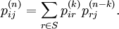
so, the n-step transition satisfies the Chapman–Kolmogorov equation, that for any k such that 0 < k < n,

$p_{ij}^{(n)} = \sum_{r \in S} p_{ir}^{(k)} p_{rj}^{(n-k)}.$

The marginal distribution Pr (X_n = x) is the distribution over states at time n. The initial distribution is Pr (X₀ = x). The evolution of the process through one time step is described by

$\Pr(X_{n}=j) = \sum_{r \in S} p_{rj} \Pr(X_{n-1}=r) = \sum_{r \in S} p_{rj}^{(n)} \Pr(X_0=r).$

The superscript $(n)$ is intended to be an integer-valued label only; however, if the Markov chain is time-homogeneous, then this superscript can also be interpreted as a "raising to the power of", discussed further below.

[edit] Reducibility

A state j is said to be accessible from a different state i (written i → j) if, given that we are in state i, there is a non-zero probability that at some time in the future, the system will be in state j. Formally, state j is accessible from state i if there exists an integer n≥0 such that

$\Pr(X_{n}=j | X_0=i) > 0.\,$

Allowing n to be zero means that every state is defined to be accessible from itself.

A state i is said to communicate with state j (written i ↔ j) if it is true that both i is accessible from j and that j is accessible from i. A set of states C is a communicating class if every pair of states in C communicates with each other, and no state in C communicates with any state not in C. (It can be shown that communication in this sense is an equivalence relation). A communicating class is closed if the probability of leaving the class is zero, namely that if i is in C but j is not, then j is not accessible from i.

Finally, a Markov chain is said to be irreducible if its state space is a communicating class; this means that, in an irreducible Markov chain, it is possible to get to any state from any state.

[edit] Periodicity

A state i has period k if any return to state i must occur in multiples of k time steps. Formally, the period of a state is defined as

$k = \operatorname{gcd}\{ n: \Pr(X_n = i | X_0 = i) > 0\}$

(where "gcd" is the greatest common divisor). Note that even though a state has period k, it may not be possible to reach the state in k steps. For example, suppose it is possible to return to the state in {6,8,10,12,...} time steps; then k would be 2, even though 2 does not appear in this list.

If k = 1, then the state is said to be aperiodic; otherwise (k>1), the state is said to be periodic with period k.

It can be shown that every state in a communicating class must have the same period.

[edit] Recurrence

A state i is said to be transient if, given that we start in state i, there is a non-zero probability that we will never return to i. Formally, let the random variable T_i be the first return time to state i (the "hitting time"):

$T_i = \inf \{ n\ge1: X_n = i | X_0 = i\}.$

Then, state i is transient if and only if:

$\Pr(T_i = {\infty}) > 0.$

If a state i is not transient (it has finite hitting time with probability 1), then it is said to be recurrent or persistent. Although the hitting time is finite, it need not have a finite expectation. Let M_i be the expected return time,

$M_i = E[T_i].\,$

Then, state i is positive recurrent if M_i is finite; otherwise, state i is null recurrent (the terms non-null persistent and null persistent are also used, respectively).

It can be shown that a state is recurrent if and only if

$\sum_{n=0}^{\infty} p_{ii}^{(n)} = \infty.$

A state i is called absorbing if it is impossible to leave this state. Therefore, the state i is absorbing if and only if

p i i = 1

and

p i j = 0

for $i \not= j.$

[edit] Ergodicity

A state i is said to be ergodic if it is aperiodic and positive recurrent. If all states in a Markov chain are ergodic, then the chain is said to be ergodic.

A finite state irreducible Markov chain is said to be ergodic if its states are aperiodic.

[edit] Regularity

A markov chain is said to be regular if there is an $n$ such that

$p_{ij}^{(n)} > 0$

for all i, j. Otherwise the chain is said to be irregular.

[edit] Steady-state analysis and limiting distributions

If the Markov chain is a time-homogeneous Markov chain, so that the process is described by a single, time-independent matrix $p i j$ , then the vector $\boldsymbol{\pi}$ is called a stationary distribution (or invariant measure) if its entries $π j$ sum to 1 and it satisfies

$\pi_j = \sum_{i \in S} \pi_i p_{ij}.$

An irreducible chain has a stationary distribution if and only if all of its states are positive recurrent. In that case, π is unique and is related to the expected return time:

$\pi_j = \frac{1}{M_j}.\,$

Further, if the chain is both irreducible and aperiodic, then for any i and j,

$\lim_{n \rarr \infty} p_{ij}^{(n)} = \frac{1}{M_j}.$

Note that there is no assumption on the starting distribution; the chain converges to the stationary distribution regardless of where it begins. Such π is called the equilibrium distribution of the chain.

If a chain is not irreducible, its stationary distributions will not be unique (consider any closed communicating class in the chain; each one will have its own unique stationary distribution. Any of these will extend to a stationary distribution for the overall chain, where the probability outside the class is set to zero). However, if a state j is aperiodic, then

$\lim_{n \rarr \infty} p_{jj}^{(n)} = \frac{1}{M_j}$

and for any other state i, let f_ij be the probability that the chain ever visits state j if it starts at i,

$\lim_{n \rarr \infty} p_{ij}^{(n)} = \frac{f_{ij}}{M_j}.$

If a state is i periodic with period k > 1 then the limit

$\lim_{n \rarr \infty} p_{ii}^{(n)}$

does not exist, although the limit

$\lim_{n \rarr \infty} p_{ii}^{(kn+r)}$

does exist for every integer r.

[edit] Markov chains with a finite state space

If the state space is finite, the transition probability distribution can be represented by a matrix, called the transition matrix, with the (i, j)th element of P equal to

$p_{ij} = \Pr(X_{n+1}=j\mid X_n=i). \,$

P is a stochastic matrix, which is an important fact to keep in mind for the rest of this discussion. If the Markov chain is time-homogeneous, then the transition matrix P is the same after each step, so the k-step transition probability can be computed as the k-th power of the transition matrix, P^k.

The stationary distribution π is a (row) vector whose entries sum to 1 that satisfies the equation

$\pi = \pi\mathbf{P}.\,$

In other words, the stationary distribution π is a normalized (meaning that the sum of its entries is 1) left eigenvector of the transition matrix associated with the eigenvalue 1.

Alternatively, π can be viewed as a fixed point of the linear (hence continuous) transformation on the unit simplex associated to the matrix P. As any continuous transformation in the unit simplex has a fixed point, a stationary distribution always exists, but is not guaranteed to be unique, in general. However, if the Markov chain is irreducible and aperiodic, then there is a unique stationary distribution π. Additionally, in this case P^k converges to a rank-one matrix in which each row is the stationary distribution π, that is,

$\lim_{k\rightarrow\infty}\mathbf{P}^k=\mathbf{1}\pi$

where 1 is the column vector with all entries equal to 1. This is stated by the Perron-Frobenius theorem. If, by whatever means, $\scriptstyle \lim_{k\to\infty}\mathbf{P}^k$ is found, then the stationary distribution of the Markov chain in question can be easily determined for any starting distribution, as will be explained below.

Since P is a stochastic matrix, $\scriptstyle \lim_{k\to\infty}\mathbf{P}^k$ always exists. Because there are a number of different special cases to consider, the process of finding this limit can be a lengthy task. All the same, there are several general rules and guidelines to keep in mind. Let P be an n×n matrix, and define $\scriptstyle \mathbf{Q} = \lim_{k\to\infty}\mathbf{P}^k.$

It is always true that

$\mathbf{QP} = \mathbf{Q}.$

Subtracting Q from both sides and factoring then yields

$\mathbf{Q}(\mathbf{P} - \mathbf{I}_{n}) = \mathbf{0}_{n,n}$

where I_n is the identity matrix of size n, and 0_n,n is the zero matrix of size n×n. Multiplying together stochastic matrices always yields another stochastic matrix, so Q must be a stochastic matrix. It is sometimes sufficient to use the matrix equation above and the fact that Q is a stochastic matrix to solve for Q.

Here is one method for doing so: first, define the function f(A) to return the matrix A with its right-most column replaced with all 1's. Then evaluate the following equation:^{[citation needed]}

$\mathbf{Q}=f(\mathbf{0}_{n,n})[f(\mathbf{P}-\mathbf{I}_n)]^{-1}.$

This equation does not work when [f(P – I_n)]^–1 does not exist. If this is the case, then it is necessary to take into account more information in order to find Q. One thing to notice is that if P has an element P_i,i on its main diagonal that is equal to 1 and the ith row or column is otherwise filled with 0's, then that row or column will remain unchanged in all of the subsequent powers P^k. Hence, the ith row or column of Q will have the 1 and the 0's in the same positions as in P.

In most cases, P^k approaches but never actually equals its limit. There are numerous exceptions to this, however, such as the case in which

$\mathbf{P} = \begin{bmatrix} 0 & 0 & 1 \\ 0 & 0 & 1 \\ 0 & 0 & 1 \end{bmatrix}.$

Then P^k = P for all k, so Q = P. Note that for any initial distribution A₀, all subsequent distributions will be

$\mathbf{A_1} = \mathbf{A_0 P} = \begin{bmatrix} 0 & 0 & 1 \end{bmatrix}.$

[edit] Reversible Markov chain

The idea of a reversible Markov chain comes from the ability to "invert" a conditional probability using Bayes' Rule:

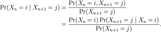
$\begin{align} \Pr(X_{n}=i\mid X_{n+1}=j) & = \frac{\Pr(X_n = i, X_{n+1} = j)}{\Pr(X_{n+1} = j)} \\ & = \frac{\Pr(X_{n} = i)\Pr(X_{n+1} = j\mid X_n=i)}{\Pr(X_{n+1} = j)}. \end{align}$

It now appears that time has been reversed. Thus, a Markov chain is said to be reversible if there is a π such that

$\pi_i p_{ij} = \pi_j p_{ji}.\,$

This condition is also known as the detailed balance condition.

Summing over i gives

$\sum_i \pi_i p_{ij} = \pi_j\,$

so for reversible Markov chains, π is always a stationary distribution.

[edit] Bernoulli scheme

A Bernoulli scheme is a special case of a Markov chain where the transition probability matrix has identical rows, which means that the next state is even independent of the current state (in addition to being independent of the past states). A Bernoulli scheme with only two possible states is known as a Bernoulli process.

[edit] Markov chains with general state space

Many results for Markov chains with finite state space can be generalized to chains with uncountable state space through Harris chains. The main idea is to see if there is a point in the state space that the chain hits with probability one. Generally, it is not true for continuous state space, however, we can define sets A and B along with a positive number ε and a probability measure ρ, such that

$\text{If }\tau_A = \inf\{n\geq 0: X_n \in A\},\text{ then } P_z(\tau_A<\infty)>0\text{ for all }z.$
$\text{If }x \in A\text{ and }C\subset B,\text{ then } p(x, C)\geq \varepsilon \rho(C).$

Then we could collapse the sets into an auxiliary point α, and a recurrent Harris chain can be modified to contain α. Lastly, the collection of Harris chains is a comfortable level of generality, which is broad enough to contain a large number of interesting examples, yet restrictive enough to allow for a rich theory.

[edit] Applications

[edit] Physics

Markovian systems appear extensively in physics, particularly statistical mechanics, whenever probabilities are used to represent unknown or unmodelled details of the system, if it can be assumed that the dynamics are time-invariant, and that no relevant history need be considered which is not already included in the state description.

[edit] Testing

Several theorists have proposed the idea of the Markov chain statistical test (MCST), a method of conjoining Markov chains to form a 'Markov blanket', arranging these chains in several recursive layers ('wafering') and producing more efficient test sets — samples — as a replacement for exhaustive testing. MCSTs also have uses in temporal state-based networks; Chilukuri et al.'s paper entitled "Temporal Uncertainty Reasoning Networks for Evidence Fusion with Applications to Object Detection and Tracking" (ScienceDirect) gives an excellent background and case study for applying MCSTs to a wider range of applications.

[edit] Queueing theory

Markov chains can also be used to model various processes in queueing theory and statistics.^[2] Claude Shannon's famous 1948 paper A mathematical theory of communication, which at a single step created the field of information theory, opens by introducing the concept of entropy through Markov modeling of the English language. Such idealized models can capture many of the statistical regularities of systems. Even without describing the full structure of the system perfectly, such signal models can make possible very effective data compression through entropy coding techniques such as arithmetic coding. They also allow effective state estimation and pattern recognition. The world's mobile telephone systems depend on the Viterbi algorithm for error-correction, while hidden Markov models are extensively used in speech recognition and also in bioinformatics, for instance for coding region/gene prediction. Markov chains also play an important role in reinforcement learning.

[edit] Internet applications

The PageRank of a webpage as used by Google is defined by a Markov chain.^[3] It is the probability to be at page $i$ in the stationary distribution on the following Markov chain on all (known) webpages. If $N$ is the number of known webpages, and a page $i$ has $k i$ links then it has transition probability $\frac{\alpha}{k_i} + \frac{1-\alpha}{N}$ for all pages that are linked to and $\frac{1-\alpha}{N}$ for all pages that are not linked to. The parameter $α$ is taken to be about 0.85.^{[citation needed]}

Markov models have also been used to analyze web navigation behavior of users. A user's web link transition on a particular website can be modeled using first- or second-order Markov models and can be used to make predictions regarding future navigation and to personalize the web page for an individual user.

[edit] Statistical

Markov chain methods have also become very important for generating sequences of random numbers to accurately reflect very complicated desired probability distributions, via a process called Markov chain Monte Carlo (MCMC). In recent years this has revolutionised the practicability of Bayesian inference methods, allowing a wide range of posterior distributions to be simulated and their parameters found numerically.

[edit] Economics

Dynamic macroeconomics heavily uses Markov chains. An example is using Markov chains to exogenously model prices of equity (stock) in a general equilibrium setting.^[4]

[edit] Social sciences

Markov chains are generally used in describing path-dependent arguments, where current structural configurations condition future outcomes. An example is the commonly argued link between economic development and the rise of democracy. Once a country reaches a specific level of economic development, the configuration of structural factors, such as size of the commercial bourgeoisie, the ratio of urban to rural residence, the rate of political mobilization, etc, will generate a higher probability of transitioning from authoritarian to democratic rule.

[edit] Mathematical biology

Markov chains also have many applications in biological modelling, particularly population processes, which are useful in modelling processes that are (at least) analogous to biological populations. The Leslie matrix is one such example, though some of its entries are not probabilities (they may be greater than 1). Another important example is the modeling of cell shape in dividing sheets of epithelial cells. The distribution of shapes – predominantly hexagonal – was a long standing mystery until it was explained by a simple Markov Model, where a cell's state is its number of sides. Empirical evidence from frogs, fruit flies, and hydra further suggests that the stationary distribution of cell shape is exhibited by almost all multicellular animals.^[5] Yet another example is the state of Ion channels in cell membranes.

[edit] Gambling

Markov chains can be used to model many games of chance. The children's games Snakes and Ladders and "Hi Ho! Cherry-O", for example, are represented exactly by Markov chains. At each turn, the player starts in a given state (on a given square) and from there has fixed odds of moving to certain other states (squares).

[edit] Music

Markov chains are employed in algorithmic music composition, particularly in software programs such as CSound or Max. In a first-order chain, the states of the system become note or pitch values, and a probability vector for each note is constructed, completing a transition probability matrix (see below). An algorithm is constructed to produce and output note values based on the transition matrix weightings, which could be MIDI note values, frequency (Hz), or any other desirable metric.

1st-order matrix
Note	A	C#	Eb
A	0.1	0.6	0.3
C#	0.25	0.05	0.7
Eb	0.7	0.3	0

2nd-order matrix
Note	A	D	G
AA	0.18	0.6	0.22
AD	0.5	0.5	0
AG	0.15	0.75	0.1
DD	0	0	1
DA	0.25	0	0.75
DG	0.9	0.1	0
GG	0.4	0.4	0.2
GA	0.5	0.25	0.25
GD	1	0	0

A second-order Markov chain can be introduced by considering the current state and also the previous state, as indicated in the second table. Higher, nth-order chains tend to "group" particular notes together, while 'breaking off' into other patterns and sequences occasionally. These higher-order chains tend to generate results with a sense of phrasal structure, rather than the 'aimless wandering' produced by a first-order system.^[6]

[edit] Baseball

Markov chain models have been used in advanced baseball analysis since 1960, although their use is still rare. Each half-inning of a baseball game fits the Markov chain state when the number of runners and outs are considered. For each half-inning there are 24 possible run-out combinations. Markov chain models can be used to evaluate runs created for both individual players as well as a team.^[7]

[edit] Markov text generators

Markov processes can also be used to generate superficially "real-looking" text given a sample document: they are used in a variety of recreational "parody generator" software (see dissociated press, Jeff Harrison, Mark V Shaney^[8] ^[9] ).

These processes are also used by spammers to inject real-looking hidden paragraphs into unsolicited email in an attempt to get these messages past spam filters.

[edit] History

Andrey Markov produced the first results (1906) for these processes, purely theoretically. A generalization to countably infinite state spaces was given by Kolmogorov (1936). Markov chains are related to Brownian motion and the ergodic hypothesis, two topics in physics which were important in the early years of the twentieth century, but Markov appears to have pursued this out of a mathematical motivation, namely the extension of the law of large numbers to dependent events. In 1913, he applied his findings for the first time to the first 20,000 letters of Pushkin's "Eugene Onegin".

Seneta^[10] provides an account of Markov's motivations and the theory's early development. The term "Markov chain" was used by Markov (1906).^[11]

[edit] See also

[edit] References

^ S. P. Meyn and R.L. Tweedie, 2005. Markov Chains and Stochastic Stability. Second edition to appear, Cambridge University Press, 2008.
^ ^a ^b S. P. Meyn, 2007. Control Techniques for Complex Networks, Cambridge University Press, 2007.
^ U.S. Patent 6,285,999
^ Brennan, Michael, and Yihong Xiab. Stock Price Volatility and the Equity Premium. Department of Finance, the Anderson School of Management, UCLA. http://bbs.cenet.org.cn/uploadImages/200352118122167693.pdf
^ http://www.eecs.harvard.edu/~abpatel/drosophila_wing_model.htm
^ Curtis Roads (ed.) (1996). The Computer Music Tutorial. MIT Press. ISBN 0262181584.
^ Pankin, Mark D.. "MARKOV CHAIN MODELS: THEORETICAL BACKGROUND". http://www.pankin.com/markov/theory.htm. Retrieved on 2007-11-26.
^ Kenner, Hugh; O'Rourke, Joseph (November 1984), "A Travesty Generator for Micros", BYTE 9 (12): 129–131, 449–469
^ Hartman, Charles (1996), The Virtual Muse: Experiments in Computer Poetry, Hanover, NH: Wesleyan University Press, ISBN 0819522392
^ Seneta, E. (1996) Markov and the Birth of Chain Dependence Theory. International Statistical Review, 64(3), 255%–263
^ Upton, G., Cook, I. (2008) Oxford Dictionary of Statistics, OUP, ISBN 0-19-954145-4

A.A. Markov. "Rasprostranenie zakona bol'shih chisel na velichiny, zavisyaschie drug ot druga". Izvestiya Fiziko-matematicheskogo obschestva pri Kazanskom universitete, 2-ya seriya, tom 15, pp 135–156, 1906.

A.A. Markov. "Extension of the limit theorems of probability theory to a sum of variables connected in a chain". reprinted in Appendix B of: R. Howard. Dynamic Probabilistic Systems, volume 1: Markov Chains. John Wiley and Sons, 1971.

Classical Text in Translation: A. A. Markov, An Example of Statistical Investigation of the Text Eugene Onegin Concerning the Connection of Samples in Chains, trans. David Link. Science in Context 19.4 (2006): 591-600. Online: http://journals.cambridge.org/production/action/cjoGetFulltext?fulltextid=637500

Leo Breiman. Probability. Original edition published by Addison-Wesley, 1968; reprinted by Society for Industrial and Applied Mathematics, 1992. ISBN 0-89871-296-3. (See Chapter 7.)

J.L. Doob. Stochastic Processes. New York: John Wiley and Sons, 1953. ISBN 0-471-52369-0.

S. P. Meyn and R. L. Tweedie. Markov Chains and Stochastic Stability. London: Springer-Verlag, 1993. ISBN 0-387-19832-6. online: http://decision.csl.uiuc.edu/~meyn/pages/book.html . Second edition to appear, Cambridge University Press, 2009.

S. P. Meyn. Control Techniques for Complex Networks. Cambridge University Press, 2007. ISBN-13: 9780521884419. Appendix contains abridged Meyn & Tweedie. online: http://decision.csl.uiuc.edu/~meyn/pages/CTCN/CTCN.html

Booth, Taylor L. (1967). Sequential Machines and Automata Theory (1st ed.). New York: John Wiley and Sons, Inc.. Library of Congress Card Catalog Number 67-25924. Extensive, wide-ranging book meant for specialists, written for both theoretical computer scientists as well as electrical engineers. With detailed explanations of state minimization techniques, FSMs, Turing machines, Markov processes, and undecidability. Excellent treatment of Markov processes pp.449ff. Discusses Z-transforms, D transforms in their context.

Kemeny, John G.; Hazleton Mirkil, J. Laurie Snell, Gerald L. Thompson (1959). Finite Mathematical Structures (1st ed.). Englewood Cliffs, N.J.: Prentice-Hall, Inc.. Library of Congress Card Catalog Number 59-12841. Classical text. cf Chapter 6 Finite Markov Chains pp.384ff.

E. Nummelin. "General irreducible Markov chains and non-negative operators". Cambridge University Press, 1984, 2004. ISBN 0-521-60494-X

[edit] Further reading

Diaconis, Persi, "The Markov chain Monte Carlo revolution", Bull. Amer. Math. Soc. (2008)

[edit] External links

Techniques to Understand Computer Simulations: Markov Chain Analysis
(pdf) Markov Chains chapter in American Mathematical Society's introductory probability book
Generates random parodies in the style of another body of text using a Markov chain algorithm
A generator that uses Markov Chains to create random words
Markov Chains
Class structure on PlanetMath
Chapter 5: Markov Chain Models
Generating Text (About generating random text using a Markov chain.)
Markov modeling tool(MEADEP)
The World's Largest Matrix Computation (Google's PageRank as the stationary distribution of a random walk through the Web.)
Dissociated Press in Emacs approximates a Markov process
Markov Chain Example
Markov Chains for Search Engines
Steganography proof-of-concept using Markov Chains.
n^th order Markov Chain implementation in Ruby
Baseball Run Modeler using Markov Chains
Theory of Markov chains in baseball
Sequential analysis software for generating visual representations of probability models

[MCSS-0] S. P. Meyn and R.L. Tweedie, 2005. Markov Chains and Stochastic Stability. Second edition to appear, Cambridge University Press, 2008.

[CTCN-1] S. P. Meyn, 2007. Control Techniques for Complex Networks, Cambridge University Press, 2007.

[2] U.S. Patent 6,285,999

[3] Brennan, Michael, and Yihong Xiab. Stock Price Volatility and the Equity Premium. Department of Finance, the Anderson School of Management, UCLA. http://bbs.cenet.org.cn/uploadImages/200352118122167693.pdf

[4] ttp://www.eecs.harvard.edu/~abpatel/drosophila_wing_model.htm

[Roads-5] Curtis Roads (ed.) (1996). The Computer Music Tutorial. MIT Press. ISBN 0262181584.

[6] Pankin, Mark D.. "MARKOV CHAIN MODELS: THEORETICAL BACKGROUND". http://www.pankin.com/markov/theory.htm. Retrieved on 2007-11-26.

[Travesty-7] Kenner, Hugh; O'Rourke, Joseph (November 1984), "A Travesty Generator for Micros", BYTE 9 (12): 129–131, 449–469

[Hartman-8] Hartman, Charles (1996), The Virtual Muse: Experiments in Computer Poetry, Hanover, NH: Wesleyan University Press, ISBN 0819522392

[9] Seneta, E. (1996) Markov and the Birth of Chain Dependence Theory. International Statistical Review, 64(3), 255%–263

[10] Upton, G., Cook, I. (2008) Oxford Dictionary of Statistics, OUP, ISBN 0-19-954145-4

[1]

[2]

[3]

[4]

[5]

[6]

[7]

[8]

[9]

[10]

[11]