Extended Euclidean algorithm
From Wikipedia, the free encyclopedia
The extended Euclidean algorithm is an extension to the Euclidean algorithm for finding the greatest common divisor (GCD) of integers a and b: it also finds the integers x and y in Bézout's identity
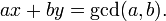
(Typically either x or y is negative).
The extended Euclidean algorithm is particularly useful when a and b are coprime, since x is the modular multiplicative inverse of a modulo b.
Contents |
[edit] Informal formulation of the algorithm
| Dividend | Divisor | Quotient | Remainder |
|---|---|---|---|
| 120 | 23 | 5 | 5 |
| 23 | 5 | 4 | 3 |
| 5 | 3 | 1 | 2 |
| 3 | 2 | 1 | 1 |
| 2 | 1 | 2 | 0 |
It is assumed that the reader is already familiar with Euclid's algorithm.
To illustrate the extension of the Euclid's algorithm, consider the computation of gcd(120, 23), which is shown on the table on the left. Notice that the quotient in each division is recorded as well alongside the remainder.
In this case, the remainder in the fourth line (which is equal to 1) indicates that the gcd is 1; that is, 120 and 23 are coprime (also called relatively prime). For the sake of simplicity, the example chosen is a coprime pair; but the more general case of gcd other than 1 also works similarly.
There are two methods to proceed, both using the division algorithm, which will be discussed separately.
[edit] The iterative method
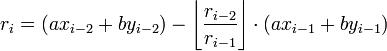
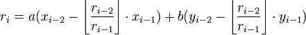
This method computes expressions of the form ri = axi + byi for the remainder in each step i of the Euclidean algorithm. Each modulus can be written in terms of the previous two remainders and their whole quotient as follows:

By substitution, this gives:
The first two values are the initial arguments to the algorithm:
- r1 = a = a(1) + b(0)
- r2 = b = a(0) + b(1)
The expression for the last non-zero remainder gives the desired results since this method computes every remainder in terms of a and b, as desired.
Example: Compute the GCD of 120 and 23.
The computation proceeds as follows:
| Step | Quotient | Remainder | Substitute | Combine terms | |
|---|---|---|---|---|---|
| 1 | 120 | 120 = 120 * 1 + 23 * 0 | |||
| 2 | 23 | 23 = 120 * 0 + 23 * 1 | |||
| 3 | 5 | 5 = 120 - 23 * 5 | 5 = (120 * 1 + 23 * 0) - (120 * 0 + 23 * 1) * 5 | 5 = 120 * 1 + 23 * -5 | |
| 4 | 4 | 3 = 23 - 5 * 4 | 3 = (120 * 0 + 23 * 1) - (120 * 1 + 23 * -5) * 4 | 3 = 120 * -4 + 23 * 21 | |
| 5 | 1 | 2 = 5 - 3 * 1 | 2 = (120 * 1 + 23 * -5) - (120 * -4 + 23 * 21) * 1 | 2 = 120 * 5 + 23 * -26 | |
| 6 | 1 | 1 = 3 - 2 * 1 | 1 = (120 * -4 + 23 * 21) - (120 * 5 + 23 * -26) * 1 | 1 = 120 * -9 + 23 * 47 | |
| 7 | 2 | 0 | End of algorithm | ||
The last line reads 1 = −9×120 + 47×23, which is the required solution: x = −9 and y = 47.
This also means that −9 is the multiplicative inverse of 120 modulo 23, and that 47 is the multiplicative inverse of 23 modulo 120.
- −9 × 120 ≡ 1 mod 23 and also 47 × 23 ≡ 1 mod 120.
[edit] The recursive method
This method attempts to solve the original equation directly, by reducing the dividend and divisor gradually, from the first line to the last line, which can then be substituted with trivial value and work backward to obtain the solution.
Consider the original equation:
| 120 | x | + | 23 | y | = | 1 |
| (5×23+5) | x | + | 23 | y | = | 1 |
| 23 | (5x+y) | + | 5 | x | = | 1 |
| ... | ||||||
| 1 | a | + | 0 | b | = | 1 |
Notice that the equation remains unchanged after decomposing the original dividend in terms of the divisor plus a remainder, and then regrouping terms. If we have a solution to the equation in the second line, then we can work backward to find x and y as required. Although we don't have the solution yet to the second line, notice how the magnitude of the terms decreased (120 and 23 to 23 and 5). Hence, if we keep applying this, eventually we'll reach the last line, which obviously has (1,0) as a trivial solution. Then we can work backward and gradually find out x and y.
| Dividend | = | Quotient | x | Divisor | + | Remainder |
|---|---|---|---|---|---|---|
| 120 | = | 5 | x | 23 | + | 5 |
| 23 | = | 4 | x | 5 | + | 3 |
| ... | ||||||
For the purpose of explaining this method, the full working will not be shown. Instead some of the repeating steps will be described to demonstrate the principle behind this method.
Start by rewriting each line from the first table with division algorithm, focusing on the dividend this time (because we'll be substituting the dividend).
| 120 | x0 | + | 23 | y0 | = | 1 |
| (5×23+5) | x0 | + | 23 | y0 | = | 1 |
| 23 | (5x0+y0) | + | 5 | x0 | = | 1 |
| 23 | x1 | + | 5 | y1 | = | 1 |
| (4×5+3) | x1 | + | 5 | y1 | = | 1 |
| 5 | (4x1+y1) | + | 3 | x1 | = | 1 |
| 5 | x2 | + | 3 | y2 | = | 1 |
|
[edit] The table method
The table method, also known as "The Magic Box", is probably the simplest method to carry out with a pencil and paper. It is similar to the recursive method, although it does not directly require algebra to use and only requires working in one direction. The main idea is to think of the equation chain

as a sequence of divisors 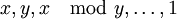 . In the running example we have the sequence 120, 23, 5, 3, 2, 1. Any element in this chain can be written as a linear combination of the original x and y, most notably, the last element, gcd(x,y), can be written in this way. The table method involves keeping a table of each divisor, written as a linear combination. The algorithm starts with the table as follows:
-
a b d 1 0 120 0 1 23
The elements in the d column of the table will be the divisors in the sequence. Each di can be represented as the linear combination
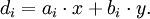
The a and b values are obvious for the first two rows of the table, which represent x and y themselves. To compute di for any i > 2, notice that

Suppose  . Then it must be that
 and
and .
.
This is easy to verify algebraically with a simple substitution.
Actually carrying out the table method though is simpler than the above equations would indicate. To find the third row of the table in the example, just notice that 120 divided by 23 goes 5 times plus a remainder. This gives us k, the multiplying factor for this row. Now, each value in the table is the value two rows above it, minus k times the value immediately above it. This correctly leads to
 ,
, , and
, and .
.
After repeating this method to find each line of the table (note that the remainder written in the table and the multiplying factor are two different numbers!), the final values for a and b will solve 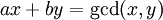 :
:
-
a b d k 1 0 120 0 1 23 5 1 -5 5 4 -4 21 3 1 5 -26 2 1 -9 47 1 2
This method is simple, requiring only the repeated application of one rule, and leaves the answer in the final row of the table with no backtracking. Note also that if you end up with a negative number as the answer for the factor of, in this case b, you will then need to add the modulus in order to make it work as a modular inverse (instead of just taking the absolute value of b). I.e. if it returns a negative number, don't just flip the sign, but add in the other number to make it work. Otherwise it will give you the modular inverse yielding negative one. If negative modular inverses still confuse you, please see this for a better explanation.
[edit] Formal description of the algorithm
[edit] Iterative method
By routine algebra of expanding and grouping like terms (refer to last section), the following algorithm for iterative method is obtained:
- Apply Euclidean algorithm, and let qn(n starts from 1) be a finite list of quotients in the division.
- Initialize x0, x1 as 1, 0, and y0, y1 as 0,1 respectively.
- Then for each i so long as qi is defined,
- Compute xi+1= xi-1- qixi
- Compute yi+1= yi-1- qiyi
- Repeat the above after incrementing i by 1.
- The answers are the second-to-last of xn and yn.
Pseudocode for this method is shown below:
function extended_gcd(a, b)
    x := 0    lastx := 1
    y := 1    lasty := 0
    while b ≠ 0
        quotient := a div b

        temp := b
        b := a mod b
        a := temp

        temp := x
        x := lastx-quotient*x
        lastx := temp

        temp := y
        y := lasty-quotient*y
        lasty := temp
    return {lastx, lasty, a}
[edit] Recursive method
Solving the general case of the equation in the last corresponding section, the following algorithm results:
- If a is divisible by b, the algorithm ends and return the trivial solution x = 0, y = 1.
- Otherwise, repeat the algorithm with b and a modulus b, storing the solution as x' and y'.
- Then, the solution to the current equation is x = y', and y = x' minus y' times quotient of a divided by b
Which can be directly translated to this pseudocode:
function extended_gcd(a, b)
    if a mod b = 0
        return {0, 1}
    else
        {x, y} := extended_gcd(b, a mod b)
        return {y, x-y*(a div b)}
[edit] Proof of correctness
Let d be the gcd of a and b. We wish to prove that a*x + b*y = d.
- If b evenly divides a (i.e. a mod b = 0),
- then d is b and a*0 + b*1 = d.
- So x and y are 0 and 1.
- Otherwise given the recursive call we know that b*x + (a mod b) * y = d,
- then b*x - b*(a div b)*y + (a mod b) * y + b*(a div b)*y= d,
- and b*(x - (a div b)*y) + a*y=d.
- So the new x and y are y and x - (a div b)*y.
See the Euclidean algorithm for the proof that the gcd(a,b) = gcd(b,a mod b) which this proof depends on in the recursive call step.
[edit] Computing a multiplicative inverse in a finite field
The extended Euclidean algorithm can also be used to calculate the multiplicative inverse in a finite field.
[edit] Pseudocode
Given the irreducible polynomial f(x) used to define the finite field, and the element a(x) whose inverse is desired, then a form of the algorithm suitable for determining the inverse is given by the following. NOTE: remainder() and quotient() are functions different from the arrays remainder[ ] and quotient[ ]. remainder() refers to the remainder when two numbers are divided, and quotient() refers to the integer quotient when two numbers are divided. For example, remainder(5/3) = 2 and quotient(5/3) = 1. Equivalent operators in the C language are % and / respectively.
remainder[1] := f(x)
remainder[2] := a(x)
auxiliary[1] := 0
auxiliary[2] := 1
i := 2
while remainder[i] > 1
    i := i + 1
    remainder[i] := remainder(remainder[i-2] / remainder[i-1])
    quotient[i] := quotient(remainder[i-2] / remainder[i-1])
    auxiliary[i] := -quotient[i] * auxiliary[i-1] + auxiliary[i-2]
inverse := auxiliary[i]
[edit] Note
The minus sign is not necessary for some finite fields in the step.
auxiliary[i] := -quotient[i] * auxiliary[i-1] + auxiliary[i-2]
This is true since in the finite field GF(28), for instance, addition and subtraction are the same. In other words, 1 is its own additive inverse in GF(28). This occurs in any finite field GF(2n), where n is an integer.
[edit] Example
For example, if the polynomial used to define the finite field GF(28) is f(x) = x8 + x4 + x3 + x + 1, and x6 + x4 + x + 1 = {53} in big-endian hexadecimal notation, is the element whose inverse is desired, then performing the algorithm results in the following:
| i | remainder[i] | quotient[i] | auxiliary[i] |
|---|---|---|---|
| 1 | x8 + x4 + x3 + x + 1 | 0 | |
| 2 | x6 + x4 + x + 1 | 1 | |
| 3 | x2 | x2 + 1 | x2 + 1 |
| 4 | x + 1 | x4 + x2 | x6 + |
| 5 | 1 | x + 1 | x7 + x6 + x3 + |
- Note: Addition in a binary finite field is XOR.
Thus, the inverse is x7 + x6 + x3 + x = {CA}, as can be confirmed by multiplying the two elements together.
[edit] The case of more than 2 numbers
One can handle the case of more than 2 numbers iteratively. First we show that gcd(a,b,c) = gcd(gcd(a,b),c). To prove this let d = gcd(a,b,c). By definition of gcd d is a divisor of a and b. Thus gcd(a,b) = kd for some k. Similarly d is a divisor of c so c = jd for some j. Let u = gcd(k,j). By our construction of u, ud | a,b,c but since d is the greatest divisor u is a unit. And since ud = gcd(gcd(a,b),c) the result is proven.
So if na + mb = gcd(a,b) then there are x and y such that x * gcd(a,b) + y * c = gcd(a,b,c) so the final equation will be
 .
.
So then to apply to n numbers we use induction
 ,
,
with the equations following directly.
[edit] References
- Thomas H. Cormen, Charles E. Leiserson, Ronald L. Rivest, and Clifford Stein. Introduction to Algorithms, Second Edition. MIT Press and McGraw-Hill, 2001. ISBN 0-262-03293-7. Pages 859–861 of section 31.2: Greatest common divisor.
[edit] See also
[edit] External links
- How to use the algorithm by hand
- How to use the algorithm by hand
- Extended Euclidean Algorithm Applet
- Source for the form of the algorithm used to determine the multiplicative inverse in GF(2^8)
- A simple explanation of the Extended Euclidean Algorithm
- Extended Euclidean Algorithm Applet(Deutsch)
- Coding of Extended Euclidean Algoritm (and what to do in the case of negative modular inverses)
|
|||||||||||||||||

