Cross product
From Wikipedia, the free encyclopedia
In mathematics, the cross product is a binary operation on two vectors in a three-dimensional Euclidean space that results in another vector which is perpendicular to the plane containing the two input vectors. The algebra defined by the cross product is neither associative nor commutative. It contrasts with the dot product which produces a scalar result. In many engineering and physics problems, it is handy to be able to construct a perpendicular vector from two existing vectors, and the cross product provides a means for doing so. The cross product is also useful as a measure of "perpendicularness"—the magnitude of the cross product of two vectors is equal to the product of their magnitudes if they are perpendicular and scales down to zero when they are parallel. The cross product is also known as the vector product, or Gibbs vector product.
The cross product is not defined except in three or seven dimensions. Like the dot product, it depends on the metric of Euclidean space. Unlike the dot product, it also depends on the choice of orientation or "handedness". Certain features of the cross product can be generalized to other situations. For arbitrary choices of orientation, the cross product must be regarded not as a vector, but as a pseudovector. For arbitrary choices of metric, and in arbitrary dimensions, the cross product can be generalized by the exterior product of vectors, defining a two-form instead of a vector.

Contents |
[edit] Definition

The cross product of two vectors a and b is denoted by a × b. In physics, sometimes the notation a ∧ b is used[1] (mathematicians do not use this notation, to avoid confusion with the exterior product).
In a three-dimensional Euclidean space, with a right-handed coordinate system, a × b is defined as a vector c that is perpendicular to both a and b, with a direction given by the right-hand rule and a magnitude equal to the area of the parallelogram that the vectors span.
The cross product is defined by the formula[2]

where θ is the measure of the smaller angle between a and b (0° ≤ θ ≤ 180°), a and b are the magnitudes of vectors a and b, and  is a unit vector perpendicular to the plane containing a and b in the direction given by the right-hand rule as illustrated. If the vectors a and b are collinear (i.e., the angle θ between them is either 0° or 180°), by the above formula, the cross product of a and b is the zero vector 0.
The direction of the vector is given by the right-hand rule, where one simply points the forefinger of the right hand in the direction of a and the middle finger in the direction of b. Then, the vector is coming out of the thumb (see the picture on the right). Using this rule implies that the cross-product is anti-commutative, i.e., b × a = - (a × b). By pointing the forefinger toward b first, and then pointing the middle finger toward a, the thumb will be forced in the opposite direction, reversing the sign of the product vector.
Using the cross product requires the handedness of the coordinate system to be taken into account (as explicit in the definition above). If a left-handed coordinate system is used, the direction of the vector is given by the left-hand rule and points in the opposite direction.
This, however, creates a problem because transforming from one arbitrary reference system to another (e.g., a mirror image transformation from a right-handed to a left-handed coordinate system), should not change the direction of . The problem is clarified by realizing that the cross-product of two vectors is not a (true) vector, but rather a pseudovector. See cross product and handedness for more detail.
[edit] Computing the cross product
[edit] Coordinate notation
The unit vectors i, j, and k from the given orthogonal coordinate system satisfy the following equalities:
- i × j = k j × k = i k × i = j
Together with the skew-symmetry and bilinearity of the cross product, these three identities are sufficient to determine the cross product of any two vectors. In particular, the following identities are also seen to hold
- j × i = −k k × j = −i i × k = −j
- i × i = j × j = k × k = 0.
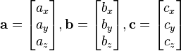
With these rules, the coordinates of the cross product of two vectors can be computed easily, without the need to determine any angles: Let
- a = a1i + a2j + a3k = (a1, a2, a3)
and
- b = b1i + b2j + b3k = (b1, b2, b3).
The cross product can be calculated by distributive cross-multiplication:
- a × b = (a1i + a2j + a3k) × (b1i + b2j + b3k)
- a × b = a1i × (b1i + b2j + b3k) + a2j × (b1i + b2j + b3k) + a3k × (b1i + b2j + b3k)
- a × b = (a1i × b1i) + (a1i × b2j) + (a1i × b3k) + (a2j × b1i) + (a2j × b2j) + (a2j × b3k) + (a3k × b1i) + (a3k × b2j) + (a3k × b3k).
Since scalar multiplication is commutative with cross multiplication, the right hand side can be regrouped as
- a × b = a1b1(i × i) + a1b2(i × j) + a1b3(i × k) + a2b1(j × i) + a2b2(j × j) + a2b3(j × k) + a3b1(k × i) + a3b2(k × j) + a3b3(k × k).
This equation is the sum of nine simple cross products. After all the multiplication is carried out using the basic cross product relationships between i, j, and k defined above,
- a × b = a1b1(0) + a1b2(k) + a1b3(−j) + a2b1(−k) + a2b2(0) + a2b3(i) + a3b1(j) + a3b2(−i) + a3b3(0).
This equation can be factored to form
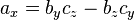
- a × b = (a2b3 − a3b2) i + (a3b1 − a1b3) j + (a1b2 − a2b1) k = (a2b3 − a3b2, a3b1 − a1b3, a1b2 − a2b1).
[edit] Matrix notation
The definition of the cross product can also be represented by the determinant of a matrix:

This determinant can be computed using Sarrus' rule. Consider the table

From the first three elements on the first row draw three diagonals sloping downward to the right (for example, the first diagonal would contain i, a2, and b3), and from the last three elements on the first row draw three diagonals sloping downward to the left (for example, the first diagonal would contain i, a3, and b2). Then multiply the elements on each of these six diagonals, and negate the last three products. The cross product would be defined by the sum of these products:

[edit] Properties
[edit] Geometric meaning
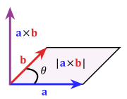

The magnitude of the cross product can be interpreted as the positive area of the parallelogram having a and b as sides (see Figure 1):

Indeed, one can also compute the volume V of a parallelepiped having a, b and c as sides by using a combination of a cross product and a dot product, called scalar triple product (see Figure 2):

Figure 2 demonstrates that this volume can be found in two ways, showing geometrically that the identity holds that a "dot" and a "cross" can be interchanged without changing the result. That is:

Because the magnitude of the cross product goes by the sine of the angle between its arguments, the cross product can be thought of as a measure of "perpendicularness" in the same way that the dot product is a measure of "parallelness". Given two unit vectors, their cross product has a magnitude of 1 if the two are perpendicular and a magnitude of zero if the two are parallel.
[edit] Algebraic properties
The cross product is anticommutative,
- a × b = −b × a,
distributive over addition,
- a × (b + c) = (a × b) + (a × c),
and compatible with scalar multiplication so that
- (r a) × b = a × (r b) = r (a × b).
It is not associative, but satisfies the Jacobi identity:
- a × (b × c) + b × (c × a) + c × (a × b) = 0.
It does not obey the cancellation law:
- If a × b = a × c and a ≠ 0 then:
- (a × b) − (a × c) = 0 and, by the distributive law above:
- a × (b − c) = 0
- Now, if a is parallel to (b − c), then even if a ≠ 0 it is possible that (b − c) ≠ 0 and therefore that b ≠ c.
However, if both a · b = a · c and a × b = a × c, then it can be concluded that b = c. Indeed,
- a · (b - c) = 0, and
- a × (b - c) = 0
so that b - c is both parallel and perpendicular to the non-zero vector a. This is only possible if b - c = 0.
The distributivity, linearity and Jacobi identity show that R3 together with vector addition and cross product forms a Lie algebra. In fact, the Lie algebra is that of the real orthogonal group in 3 dimensions, SO(3).
Further, two non-zero vectors a and b are parallel if and only if a × b = 0.
It follows from the geometrical definition above that the cross product is invariant under rotations about the axis defined by a×b.
[edit] Triple product expansion
The triple product expansion, also known as Lagrange's formula, is a formula relating the cross product of three vectors (called the vector triple product) with the dot product:
- a × (b × c) = b(a · c) − c(a · b).
The mnemonic “BAC minus CAB” is used to remember the order of the vectors in the right hand member. This formula is used in physics to simplify vector calculations. A special case, regarding gradients and useful in vector calculus, is given below.

This is a special case of the more general Laplace-de Rham operator Δ = dδ + δd.
The following identity also relates the cross product and the dot product:

This is a special case of the multiplicativity  of the norm in the quaternion algebra, and a restriction to
  of Lagrange's identity.
[edit] Alternative ways to compute the cross product
[edit] Quaternions
The cross product can also be described in terms of quaternions, and this is why the letters i, j, k are a convention for the standard basis on  : it is thought of as the imaginary quaternions.
For instance, the above given cross product relations among i, j, and k agree with the multiplicative relations among the quaternions i, j, and k. In general, if a vector [a1, a2, a3] is represented as the quaternion a1i + a2j + a3k, the cross product of two vectors can be obtained by taking their product as quaternions and deleting the real part of the result. The real part will be the negative of the dot product of the two vectors.
Alternatively and more straightforwardly, using the above identification of the 'purely imaginary' quaternions with , the cross product may be thought of as half of the commutator of two quaternions.
[edit] Conversion to matrix multiplication
A cross product between two vectors (which can only be defined in three-dimensional space) can be rewritten in terms of pure matrix multiplication as the product of a skew-symmetric matrix and a vector, as follows:
![\mathbf{a} \times \mathbf{b} = [\mathbf{a}]_{\times} \mathbf{b} = \begin{bmatrix}\,0&\!-a_3&\,\,a_2\\ \,\,a_3&0&\!-a_1\\-a_2&\,\,a_1&\,0\end{bmatrix}\begin{bmatrix}b_1\\b_2\\b_3\end{bmatrix}](http://upload.wikimedia.org/math/b/b/0/bb0828317b64e54d924e3d9dabb54234.png)
![\mathbf{a} \times \mathbf{b} = [\mathbf{b}]^T_{\times} \mathbf{a} = \begin{bmatrix}\,0&\,\,b_3&\!-b_2\\ -b_3&0&\,\,b_1\\\,\,b_2&\!-b_1&\,0\end{bmatrix}\begin{bmatrix}a_1\\a_2\\a_3\end{bmatrix}](http://upload.wikimedia.org/math/f/4/4/f44555a04678456b9390bfaa0ff9a4e4.png)
where
![[\mathbf{a}]_{\times} \stackrel{\rm def}{=} \begin{bmatrix}\,\,0&\!-a_3&\,\,\,a_2\\\,\,\,a_3&0&\!-a_1\\\!-a_2&\,\,a_1&\,\,0\end{bmatrix}.](http://upload.wikimedia.org/math/3/8/e/38e1feb99d143b91383d2fb96ce8e10f.png)
Also, if  is itself a cross product:

then
![[\mathbf{a}]_{\times} = (\mathbf{c}\mathbf{d}^T)^T - \mathbf{c}\mathbf{d}^T.](http://upload.wikimedia.org/math/5/5/d/55d46afc14c256de89aa56b17ef38491.png)
This notation provides another way of generalizing cross product to the higher dimensions by substituting pseudovectors (such as angular velocity or magnetic field) with such skew-symmetric matrices. It is clear that such physical quantities will have n(n-1)/2 independent components in n dimensions, which coincides with number of dimensions for three-dimensional space, and this is why vectors can be used (and most often are used) to represent such quantities.
This notation is also often much easier to work with, for example, in epipolar geometry.
From the general properties of the cross product follows immediately that
![[\mathbf{a}]_{\times} \, \mathbf{a} = \mathbf{0}](http://upload.wikimedia.org/math/b/0/0/b00e919750be3b08a60e4757f3cf9cf9.png) and
and ![\mathbf{a}^{T} \, [\mathbf{a}]_{\times} = \mathbf{0}](http://upload.wikimedia.org/math/7/6/2/762d1d364c16664eff7d042f99842e70.png)
and from fact that ![[\mathbf{a}]_{\times}](http://upload.wikimedia.org/math/d/0/0/d00b55ad4c7fdd0a1f2a424e0ca572ef.png) is skew-symmetric it follows that
is skew-symmetric it follows that
![\mathbf{b}^{T} \, [\mathbf{a}]_{\times} \, \mathbf{b} = 0.](http://upload.wikimedia.org/math/b/0/e/b0e7a57333b3ebbdf3c81c827152e5fa.png)
The above-mentioned triple product expansion (bac-cab rule) can be easily proven using this notation.
The above definition of means that there is a one-to-one mapping between the set of 3×3 skew-symmetric matrices, also known as the Lie algebra of SO(3), and the operation of taking the cross product with some vector .
[edit] Index notation
The cross product can alternatively be defined in terms of the Levi-Civita symbol, 

where the indices i,j,k correspond, as in the previous section, to orthogonal vector components. This characterization of the cross product is often expressed more compactly using the Einstein summation convention as

in which repeated indices are summed from 1 to 3. Note that this representation is another form of the skew-symmetric representation of the cross product:
![\varepsilon_{ijk} a_j = [\mathbf{a}]_\times](http://upload.wikimedia.org/math/6/7/8/6787bcf7f0177d3889da0246158e1398.png)
[edit] Mnemonic
The word xyzzy can be used to remember the definition of the cross product.
If

where:
then:


The second and third equations can be obtained from the first by simply vertically rotating the subscripts, x → y → z → x. The problem, of course, is how to remember the first equation, and two options are available for this purpose: either to remember the relevant two diagonals of Sarrus's scheme (those containing i), or to remember the xyzzy sequence.
Since the first diagonal in Sarrus's scheme is just the main diagonal of the above-mentioned  matrix, the first three letters of the word xyzzy can be very easily remembered.
[edit] Applications
[edit] Computational geometry
The cross product can be used to calculate the normal for a triangle or polygon, an operation frequently performed in computer graphics.
In computational geometry of the plane, the cross product is used to determine the sign of the acute angle defined by three points p1 = (x1,y1), p2 = (x2,y2) and p3 = (x3,y3). It corresponds to the direction of the cross product of the two coplanar vectors defined by the pairs of points p1,p2 and p1,p3, i.e., by the sign of the expression P = (x2 − x1)(y3 − y1) − (y2 − y1)(x3 − x1). In the "right-handed" coordinate system, if the result is 0, the points are collinear; if it is positive, the three points constitute a negative angle of rotation around p2 from p1 to p3, otherwise a positive angle. From another point of view, the sign of P tells whether p3 lies to the left or to the right of line p1,p2.
[edit] Other
The cross product occurs in the formula for the vector operator curl. It is also used to describe the Lorentz force experienced by a moving electrical charge in a magnetic field. The definitions of torque and angular momentum also involve the cross product.
The trick of rewriting a cross product in terms of a matrix multiplication appears frequently in epipolar and multi-view geometry, in particular when deriving matching constraints.
[edit] Cross product as an exterior product

The cross product can be viewed in terms of the exterior product. This view allows for a natural geometric interpretation of the cross product. In exterior calculus the exterior product (or wedge product) of two vectors is a bivector. A bivector is an oriented plane element, in much the same way that a vector is an oriented line element. Given two vectors a and b, one can view the bivector a∧b as the oriented parallelogram spanned by a and b. The cross product is then obtained by taking the Hodge dual of the bivector a∧b, identifying 2-vectors with vectors:

This can be thought of as the oriented multi-dimensional element "perpendicular" to the bivector. Only in three dimensions is the result an oriented line element – a vector – whereas, for example, in 4 dimensions the Hodge dual of a bivector is two-dimensional – another oriented plane element. So, in three dimensions only is the cross product of a and b the vector dual to the bivector a∧b: it is perpendicular to the bivector, with orientation dependent on the coordinate system's handedness, and has the same magnitude relative to the unit normal vector as a∧b has relative to the unit bivector; precisely the properties described above.
[edit] Cross product and handedness
When measurable quantities involve cross products, the handedness of the coordinate systems used cannot be arbitrary. However, when physics laws are written as equations, it should be possible to make an arbitrary choice of the coordinate system (including handedness). To avoid problems, one should be careful to never write down an equation where the two sides do not behave equally under all transformations that need to be considered. For example, if one side of the equation is a cross product of two vectors, one must take into account that when the handedness of the coordinate system is not fixed a priori, the result is not a (true) vector but a pseudovector. Therefore, for consistency, the other side must also be a pseudovector.[citation needed]
More generally, the result of a cross product may be either a vector or a pseudovector, depending on the type of its operands (vectors or pseudovectors). Namely, vectors and pseudovectors are interrelated in the following ways under application of the cross product:
-
- vector × vector = pseudovector
- vector × pseudovector = vector
- pseudovector × pseudovector = pseudovector
Because the cross product may also be a (true) vector, it may not change direction with a mirror image transformation. This happens, according to the above relationships, if one of the operands is a (true) vector and the other one is a pseudovector (e.g., the cross product of two vectors). For instance, a vector triple product involving three (true) vectors is a (true) vector.
A handedness-free approach is possible using exterior algebra.
[edit] Generalizations
There are several ways to generalize the cross product to the higher dimensions.
[edit] Lie algebra
The cross product can be seen as one of the simplest Lie products, and is thus generalized by Lie algebras, which are axiomatized as binary products satisfying the axioms of multilinearity, skew-symmetry, and the Jacobi identity. Many Lie algebras exist, and their study is a major field of mathematics, called Lie theory.
For example, the Heisenberg algebra gives another Lie algebra structure on  In the basis {x,y,z}, the product is [x,y] = z,[x,z] = [y,z] = 0.
[edit] Using octonions
A cross product for 7-dimensional vectors can be obtained in the same way by using the octonions instead of the quaternions. The nonexistence of such cross products of two vectors in other dimensions is related to the result that the only normed division algebras are the ones with dimension 1, 2, 4, and 8.
[edit] Wedge product
In general dimension, there is no direct analogue of the binary cross product. There is however the wedge product, which has similar properties, except that the wedge product of two vectors is now a 2-vector instead of an ordinary vector. As mentioned above, the cross product can be interpreted as the wedge product in three dimensions after using Hodge duality to identify 2-vectors with vectors.
The wedge product and dot product can be combined to form the Clifford product.
[edit] Multilinear algebra
In the context of multilinear algebra, the cross product can be seen as the (1,2)-tensor (a mixed tensor) obtained from the 3-dimensional volume form,[note 1] a (0,3)-tensor, by raising an index.
In detail, the 3-dimensional volume form defines a product 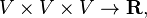 by taking the determinant of the matrix given by these 3 vectors. By duality, this is equivalent to a function
  (fixing any two inputs gives a function
  by evaluating on the third input) and in the presence of an inner product (such as the dot product; more generally, a non-degenerate bilinear form), we have an isomorphism
  and thus this yields a map
  which is the cross product: a (0,3)-tensor (3 vector inputs, scalar output) has been transformed into a (1,2)-tensor (2 vector inputs, 1 vector output) by "raising an index".
Translating the above algebra into geometry, the function "volume of the parallelepiped defined by (a,b, − )" (where the first two vectors are fixed and the last is an input), which defines a function , can be represented uniquely as the dot product with a vector: this vector is the cross product  From this perspective, the cross product is defined by the scalar triple product,
In the same way, in higher dimensions one may define generalized cross products by raising indices of the n-dimensional volume form, which is a (0,n)-tensor. The most direct generalizations of the cross product are to define either:
- a (1,n − 1)-tensor, which takes as input n − 1 vectors, and gives as output 1 vector – an (n − 1)-ary vector-valued product, or
- a (n − 2,2)-tensor, which takes as input 2 vectors and gives as output skew-symmetric tensor of rank n−2 – a binary product with rank n−2 tensor values.
One can also define (k,n − k)-tensors for other k.
These products are all multilinear and skew-symmetric, and can be defined in terms of the determinant and parity.
The (n − 1)-ary product can be described as follows: given n − 1 vectors  in
in  define their generalized cross product
  as:
as:
- perpendicular to the hyperplane defined by the vi,
- magnitude is the volume of the parallelotope defined by the vi, which can be computed as the Gram determinant of the vi,
- oriented so that

This is the unique multilinear, alternating product which evaluates to  ,
,  and so forth for cyclic permutations of indices.
In coordinates, one can give a formula for this n-ary analogue of the cross product in Rn+1 by:

This formula is identical in structure to the determinant formula for the normal cross product in R3 except that the row of basis vectors is the last row in the determinant rather than the first. The reason for this is to ensure that the ordered vectors (v1,...,vn,Λ(v1,...,vn)) have a positive orientation with respect to (e1,...,en+1). If n is even, this modification leaves the value unchanged, so this convention agrees with the normal definition of the binary product. In the case that n is odd, however, the distinction must be kept. This n-ary form enjoys many of the same properties as the vector cross product: it is alternating and linear in its arguments, it is perpendicular to each argument, and its magnitude gives the hypervolume of the region bounded by the arguments. And just like the vector cross product, it can be defined in a coordinate independent way as the Hodge dual of the wedge product of the arguments.
[edit] History
In 1773, Joseph Louis Lagrange introduced the component form of both the dot and cross products in order to study the tetrahedron in three dimensions.[3] In 1843 the Irish mathematical physicist Sir William Rowan Hamilton introduced the quaternion product, and with it the terms "vector" and "scalar". Given two quaternions [0, u] and [0, v], where u and v are vectors in R3, their quaternion product can be summarized as [−u·v, u×v]. James Clerk Maxwell used Hamilton's quaternion tools to develop his famous electromagnetism equations, and for this and other reasons quaternions for a time were an essential part of physics education.
However, Oliver Heaviside in England and Josiah Willard Gibbs in Connecticut felt that quaternion methods were too cumbersome, often requiring the scalar or vector part of a result to be extracted. Thus, about forty years after the quaternion product, the dot product and cross product were introduced — to heated opposition. Pivotal to (eventual) acceptance was the efficiency of the new approach, allowing Heaviside to reduce the equations of electromagnetism from Maxwell's original 20 to the four commonly seen today.
Largely independent of this development, and largely unappreciated at the time, Hermann Grassmann created a geometric algebra not tied to dimension two or three, with the exterior product playing a central role. William Kingdon Clifford combined the algebras of Hamilton and Grassmann to produce Clifford algebra, where in the case of three-dimensional vectors the bivector produced from two vectors dualizes to a vector, thus reproducing the cross product.
The cross notation, which began with Gibbs, inspired the name "cross product". Originally appearing in privately published notes for his students in 1881 as Elements of Vector Analysis, Gibbs’s notation — and the name — later reached a wider audience through Vector Analysis (Gibbs/Wilson), a textbook by a former student. Edwin Bidwell Wilson rearranged material from Gibbs's lectures, together with material from publications by Heaviside, Föpps, and Hamilton. He divided vector analysis into three parts:
- "First, that which concerns addition and the scalar and vector products of vectors. Second, that which concerns the differential and integral calculus in its relations to scalar and vector functions. Third, that which contains the theory of the linear vector function."
Two main kinds of vector multiplications were defined, and they were called as follows:
- The direct, scalar, or dot product of two vectors
- The skew, vector, or cross product of two vectors
Several kinds of triple products and products of more than three vectors were also examined. The above mentioned triple product expansion was also included.
[edit] See also
- Triple products — Products involving three vectors.
- Multiple cross products — Products involving more than three vectors.
- Dot product
- Cartesian product — A product of two sets.
- × (the symbol)
[edit] Notes
- ^ By a volume form one means a function that takes in n vectors and gives out a scaler, the volume of the parallelotope defined by the vectors:
 This is an n-ary multilinear skew-symmetric form. In the presence of a basis, such as on this is given by the determinant, but in an abstract vector space, this is added structure. In terms of G-structures, a volume form is an SL-structure.
[edit] References
- ^ Jeffreys, H and Jeffreys, BS (1999). Methods of mathematical physics. Cambridge University Press. http://worldcat.org/oclc/41158050?tab=details.
- ^ Wilson 1901
- ^ Lagrange, JL (1773). "Solutions analytiques de quelques problèmes sur les pyramides triangulaires". Oeuvres. vol 3.
[edit] References
- Cajori, Florian (1929), A History Of Mathematical Notations Volume II, Open Court Publishing, p. 134, ISBN 978-0-486-67766-8, http://www.archive.org/details/historyofmathema027671mbp
- Wilson, Edwin Bidwell (1901), Vector Analysis: A text-book for the use of students of mathematics and physics, founded upon the lectures of J. Willard Gibbs, Yale University Press, http://www.archive.org/details/117714283
[edit] External links
- Eric W. Weisstein, Cross Product at MathWorld.
- Z.K. Silagadze (2002). Multi-dimensional vector product. Journal of Physics. A35, 4949 (it is only possible in 7-D space)
- Real and Complex Products of Complex Numbers
- An interactive tutorial created at Syracuse University - (requires java)
- W. Kahan (2007). Cross-Products and Rotations in Euclidean 2- and 3-Space. University of California, Berkeley (PDF).
|
|||||

