IS/LM model

From Wikipedia, the free encyclopedia

This article does not cite any references or sources. Please help improve this article by adding citations to reliable sources (ideally, using inline citations). Unsourced material may be challenged and removed. (December 2007)

The IS curve moves to the right, causing higher interest rates (i) and expansion in the "real" economy (real GDP, or Y).

The IS/LM model is a macroeconomic tool that demonstrates the relationship between interest rates and real output in the goods and services market and the money market. The intersection of the IS and LM curves is the "General Equilibrium" where there is simultaneous equilibrium in all the markets of the economy^[1]. IS/LM stands for Investment Saving / Liquidity preference Money supply.

[edit] History

The IS/LM model was born at the Econometric Conference held in Oxford during September, 1936. Roy Harrod, John R. Hicks, and James Meade all presented papers describing mathematical models attempting to summarize John Maynard Keynes' General Theory of Employment, Interest, and Money. Hicks, who had seen a draft of Harrod's paper, invented the IS/LM model (originally using LL, not LM). He later presented it in "Mr. Keynes and the Classics: A Suggested Interpretation".^[2]

Hicks later agreed that the model missed important points from the Keynesian theory, criticizing it as having very limited use beyond "a classroom gadget", and criticizing equilibrium methods generally: "When one turns to questions of policy, looking towards the future instead of the past, the use of equilibrium methods is still more suspect."^[3] The first problem was that it presents the real and monetary sectors as separate, something Keynes attempted to transcend. In addition, an equilibrium model ignores uncertainty – and that liquidity preference only makes sense in the presence of uncertainty "For there is no sense in liquidity, unless expectations are uncertain."^[4] A shift in the IS or LM curve will cause change in expectations, causing the other curve to shift. Most modern macroeconomists see the IS/LM model as being at best a first approximation for understanding the real world.

Although disputed in some circles and accepted to be imperfect, the model is widely used and seen as useful in gaining an understanding of macroeconomic theory. It is used in the popular U.S. college macroeconomics textbook by Gregory Mankiw, and many others.

[edit] Formulation

The model is presented as a graph of two intersecting lines in the first quadrant.

The horizontal axis represents national income or real gross domestic product and is labelled Y. The vertical axis represents the nominal interest rate, i.

The point where these schedules intersect represents a short-run equilibrium in the real and monetary sectors (though not necessarily in other sectors, such as labor markets): both product markets and money markets are in equilibrium. This equilibrium yields a unique combination of interest rates and real GDP.

[edit] IS schedule

The IS schedule is drawn as a downward-sloping curve with interest rates as a function of GDP (Y). The initials IS stand for "Investment and Saving equilibrium" but since 1937 have been used to represent the locus of all equilibria where total spending (consumer spending + planned private investment + government purchases + net exports) equals an economy's total output (equivalent to real income, Y, or GDP). To keep the link with the historical meaning, the IS curve can represent the equilibria where total private investment equals total saving, where the latter equals consumer saving plus government saving (the budget surplus) plus foreign saving (the trade surplus). Either way, in equilibrium, all spending is desired or planned; there is no unplanned inventory accumulation (i.e., no general glut of goods and services).^[5] The level of real GDP (Y) is determined along this line for each interest rate.

Thus the IS schedule is a locus of points of equilibrium in the "real" (non-financial) economy. Given expectations about returns on fixed investment, every level of interest rate (i) will generate a certain level of planned fixed investment and other interest-sensitive spending: lower interest rates encourage higher fixed investment and the like. Income is at the equilibrium level for a given interest rate when the saving consumers choose to do out of that income equals investment (or, more generally, when "leakages" from the circular flow equal "injections"). A higher level of income is needed to generate a higher level of saving (or leakages) at a given interest rate. Alternatively, the multiplier effect of an increase in fixed investment raises real GDP. Both ways explain the downward slope of the IS schedule. In sum, this line represents the line of causation from falling interest rates to rising planned fixed investment (etc.) to rising national income and output.

In a closed economy, the IS curve is defined as: , where Y represents income, C(Y − T) represents consumer spending as a function of disposable income (income, Y, minus taxes, T), I(r) represents investment as a function of the real interest rate, and G represents government spending. In this equation, the level of G (government spending) and T (taxes) are presumed to be exogenous, meaning that they are taken as a given. To adapt this model to an open economy, a term for net exports (exports, X, minus imports, M) would need to be added to the IS equation. An economy with more imports than exports would have a negative net exports number.

[edit] LM Schedule

The LM schedule is an upward-sloping curve representing the role of finance and money. The initials LM stand for "Liquidity preference and Money supply equilibrium". As such, the LM function is the equilibrium point between the liquidity preference function and the money supply function (as determined by banks and central banks).

The liquidity preference function is simply the willingness to hold cash balances instead of securities. For this function, the interest rate (the vertical) is plotted against the quantity of cash balances (or liquidity, on the horizontal). The liquidity preference function is downward sloping. Two basic elements determine the quantity of cash balances demanded (liquidity preference) - and therefore the position and slope of the function:

• 1) Transactions demand for money: this includes both a) the willingness to hold cash for everyday transactions as well as b) as a precautionary measure - in case of emergencies. Transactions demand is positively related to real GDP (represented by Y). This is simply explained - as GDP increases, so does spending and therefore transactions. As GDP is considered exogenous to the liquidity preference function, changes in GDP shift the curve. For example, an increase in GDP will, ceteris paribus (all else equal), move the entire liquidity function rightward in proportion to the GDP increase.
• 2) Speculative demand for money: this is the willingness to hold cash as an asset for speculative purposes. Speculative demand is inversely related to the interest rate. As the interest rate rises, the opportunity cost of holding cash increases - the incentive will be to move into securities. As will expectations based on current interest rate trends contributes to the inverse relationship. As the interest rate rises above its historical value, the expectation is for the interest rate to drop. Thus the incentive is to move out of securities and into cash.

The money supply function for this situation is plotted on the same graph as the liquidity preference function. Money supply is determined by the central bank decisions and willingness of commercial banks to loan money. Though the money supply is related indirectly to interest rates, in the short run, money supply in effect perfectly inelastic with respect to nominal interest rates. Thus the money supply function is represented as a vertical line - it is a constant, independent of the interest rate GDP and other factors. Mathematically, the LM curve is defined as M / P = L(r,Y), where the supply of money is represented as the real money balance M/P (as opposed to the nominal balance M), with P representing the price level, equals the demand for money L, which is some function of the interest rate and the level of income.

Holding all variables constant, the intersection point between the liquidity preference and money supply functions constitute a single point on the LM curve. Recalling that for the LM curve, interest rate is plotted against the real GDP whereas the liquidity preference and money supply functions plot interest rates against quantity of cash balances), that an increase in GDP shifts the liquidity preference function rightward and that the money supply is constant, independent of GDP - the shape of the LM function becomes clear. As GDP increases, the negatively sloped liquidity preference function shifts rightward. Money supply, and therefore cash balances, are constant and thus, the interest rate increases. It is easy to see therefore, that the LM function is positively sloped.

[edit] Shifts

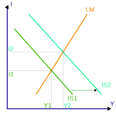
One hypothesis is that a government's deficit spending ("fiscal policy") has an effect similar to that of a lower saving rate or increased private fixed investment, increasing the amount of aggregate demand for national income at each individual interest rate. An increased deficit by the national government shifts the IS curve to the right. This raises the equilibrium interest rate (from i₁ to i₂) and national income (from Y₁ to Y₂), as shown in the graph above.

From the point of view of quantity theory of money, fiscal actions that leave the money supply unchanged can only shift aggregate demand if they receive support from the monetary sector. In this case, the velocity or demand of money determines aggregate demand. If the velocity of money remains unchanged at the initial level of output, so does aggregate demand. Essentially, the monetary sector is the source of any shift that occurs.^[6]

The graph indicates one of the major criticisms of deficit spending as a way to stimulate the economy: rising interest rates lead to crowding out – i.e., discouragement – of private fixed investment, which in turn may hurt long-term growth of the supply side (potential output). Keynesians respond that deficit spending may actually "crowd in" (encourage) private fixed investment via the accelerator effect, which helps long-term growth. Further, if government deficits are spent on productive public investment (e.g., infrastructure or public health) that directly and eventually raises potential output.

The IS/LM model also allows for the role of monetary policy. If the money supply is increased, that shifts the LM curve to the right, lowering interest rates and raising equilibrium national income.

Usually the model is used to study the short run when prices are fixed or sticky and no inflation is taken into consideration. To include these and other crucial issues, several further diagrams are needed or the equations behind the curves need to be modified.

[edit] References

This article's citation style may be unclear. The references used may be clearer with a different or consistent style of citation, footnoting, or external linking.

[edit] Related Models

• AD-AS Model
• AD-IA Model
• Mundell-Fleming model

[edit] See also

• Policy-mix
• Money demand

[edit] External links

• Elmer G. Wiens: IS-LM Model - An On-line, Interactive IS-LM Model of the Canadian Economy.
• The Hicks-Hansel IS-LM Model: [2] in-depth comment and explanation.
• Krugman, Paul. There's something about macro - explaining the model and its role in understanding macroeconomics
• Weerapana, Akila. [3] - Lecture Notes explaining the IS Curve and the LM Curve