Decision tree learning
From Wikipedia, the free encyclopedia
Decision tree learning, used in data mining and machine learning, uses a decision tree as a predictive model which maps observations about an item to conclusions about the item's target value. More descriptive names for such tree models are classification trees or regression trees. In these tree structures, leaves represent classifications and branches represent conjunctions of features that lead to those classifications.
In decision theory and decision analysis, a decision tree is a graph or model of decisions and their possible consequences, including chance event outcomes, resource costs, and utility. It can be used to create a plan to reach a goal. Decision trees are constructed in order to help with making decisions. A decision tree is a special form of tree structure. Another use of trees is as a descriptive means for calculating conditional probabilities.
In decision analysis, a decision tree can be used to visually and explicitly represent decisions and decision making. In data mining, a decision tree describes data but not decisions; rather the resulting classification tree can be an input for decision making. This page deals with trees in data mining.
Contents |
[edit] General
Decision tree learning is a common method used in data mining. Each interior node corresponds to a variable; an arc to a child represents a possible value of that variable. A leaf represents a possible value of target variable given the values of the variables represented by the path from the root.
A tree can be "learned" by splitting the source set into subsets based on an attribute value test. This process is repeated on each derived subset in a recursive manner called recursive partitioning. The recursion is completed when splitting is either non-feasible, or a singular classification can be applied to each element of the derived subset. A random forest classifier uses a number of decision trees, in order to improve the classification rate.
In data mining, trees can be described also as the combination of mathematical and computing techniques to aid the description, categorisation and generalisation of a given set of data.
Data comes in records of the form:
(x, y) = (x1, x2, x3..., xk, y)
The dependent variable, Y, is the variable that we are trying to understand, classify or generalise. The other variables, x1, x2, x3 etc., are the variables that will help with that task.
[edit] Types
In data mining, trees have three more descriptive categories/names:
- Classification tree analysis is when the predicted outcome is the class to which the data belongs.
- Regression tree analysis is when the predicted outcome can be considered a real number (e.g. the price of a house, or a patient’s length of stay in a hospital).
- Classification And Regression Tree (CART) analysis is used to refer to both of the above procedures, first introduced by Breiman et al. (BFOS84).
[edit] Practical example
Our friend David is the manager of a famous golf club. Sadly, he is having some trouble with his customer attendance. There are days when everyone wants to play golf and the staff are overworked. On other days, for no apparent reason, no one plays golf and staff have too much slack time. David’s objective is to optimise staff availability by trying to predict when people will play golf. To accomplish that he needs to understand the reason people decide to play and if there is any explanation for that. He assumes that weather must be an important underlying factor, so he decides to use the weather forecast for the upcoming week. So during two weeks he has been recording:
- The outlook, whether it was sunny, overcast or raining.
- The temperature (in degrees Fahrenheit).
- The relative humidity in percent.
- Whether it was windy or not.
- Whether people attended the golf club on that day.
David compiled this dataset into a table containing 14 rows and 5 columns as shown below.

He then applied a decision tree model to solve his problem.
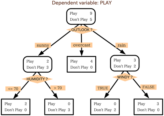
A decision tree is a model of the data that encodes the distribution of the class label (again the Y) in terms of the predictor attributes. It is a directed acyclic graph in form of a tree. The top node represents all the data. The classification tree algorithm concludes that the best way to explain the dependent variable, play, is by using the variable "outlook". Using the categories of the variable outlook, three different groups were found:
- One that plays golf when the weather is sunny,
- One that plays when the weather is cloudy, and
- One that plays when it's raining.
David's first conclusion: if the outlook is overcast people always play golf, and there are some fanatics who play golf even in the rain. Then he divided the sunny group in two. He realised that people don't like to play golf if the humidity is higher than seventy percent.
Finally, he divided the rain category in two and found that people will also not play golf if it is windy.
And lastly, here is the short solution of the problem given by the classification tree: David dismisses most of the staff on days that are sunny and humid or on rainy days that are windy, because almost no one is going to play golf on those days. On days when a lot of people will play golf, he hires extra staff. The conclusion is that the decision tree helped David turn a complex data representation into a much easier structure (parsimonious).
[edit] Formulae
[edit] Gini impurity
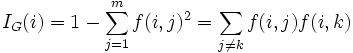
Used by the CART algorithm, Gini impurity is based on squared probabilities of membership for each target category in the node. It reaches its minimum (zero) when all cases in the node fall into a single target category.
Suppose y takes on values in {1, 2, ..., m}, and let f(i, j) = probability of getting value j in node i. That is, f(i, j) is the proportion of records assigned to node i for which y = j.
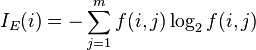
[edit] Information gain
Used by the ID3, C4.5 and C5.0 tree generation algorithms. Information gain is based on the concept of entropy used in information theory .
[edit] Decision tree advantages
Amongst other data mining methods, decision trees have several advantages:
- Simple to understand and interpret. People are able to understand decision tree models after a brief explanation.
- Requires little data preparation. Other techniques often require data normalisation, dummy variables need to be created and blank values to be removed.
- Able to handle both numerical and categorical data. Other techniques are usually specialised in analysing datasets that have only one type of variable. Ex: relation rules can be only used with nominal variables while neural networks can be used only with numerical variables.
- Use a white box model. If a given situation is observable in a model the explanation for the condition is easily explained by boolean logic. An example of a black box model is an artificial neural network since the explanation for the results is excessively complex to be comprehended.
- Possible to validate a model using statistical tests. That makes it possible to account for the reliability of the model.
- Robust, perform well with large data in a short time. Large amounts of data can be analysed using personal computers in a time short enough to enable stakeholders to take decisions based on its analysis.
[edit] Limitations
- The problem of learning an optimal decision tree is known to be NP-complete.[1] Consequently, practical decision-tree learning algorithms are based on weak (heuristic) algorithms such as the greedy algorithm where locally optimal decisions are made at each node. Such algorithms cannot guarantee to return the globally optimal decision tree.
- Decision-tree learners create over-complex trees that do not generalise the data well. This is called overfitting[2]. Mechanisms such as pruning are necessary to avoid this problem.
- There are concepts that are hard to learn because decision trees do not express them easily, such as XOR, parity or multiplexer problems. In such cases, the decision tree becomes prohibitively large. Approaches to solve the problem involve either changing the representation of the problem domain, known as propositionalisation[3] or using learning algorithms based on more expressive representations instead, such as statistical relational learning or inductive logic programming.
[edit] Extending decision trees with decision graphs
In a decision tree, all paths from the root node to the leaf node proceed by way of conjunction, or AND. In a decision graph, it is possible to use disjunctions (ORs) to join two more paths together using Minimum Message Length (MML)[4]. Decision graphs have been further extended to allow for previously unstated new attributes to be learnt dynamically and used at different places within the graph.[5] The more general coding scheme results in better predictive accuracy and log-loss probabilistic scoring. In general, decision graphs infer models with fewer leaves than decision trees.
[edit] See also
- Decision-tree pruning
- Pruning (algorithm)
- Binary decision diagram
- CART
- ID3 algorithm
- C4.5 algorithm
- Random forest
- Decision stump
[edit] External sources
- V.Berikov, A.Litvinenko, "Methods for statistical data analysis with decision trees". Novosibirsk, Sobolev Institute of Mathematics, 2003. Methods for statistical data analysis with decision trees
- [BFOS84] L. Breiman, J. Friedman, R. A. Olshen and C. J. Stone, "Classification and regression trees". Wadsworth, 1984.
- [1] T. Menzies, Y. Hu, Data Mining For Very Busy People. IEEE Computer, October 2003, pgs. 18-25.
- Decision Tree Analysis mindtools.com
- J.W. Comley and D.L. Dowe, "Minimum Message Length, MDL and Generalised Bayesian Networks with Asymmetric Languages", chapter 11 (pp265-294) in P. Grunwald, M.A. Pitt and I.J. Myung (eds)., Advances in Minimum Description Length: Theory and Applications, M.I.T. Press, April 2005, ISBN 0-262-07262-9. (This paper puts decision trees in internal nodes of Bayesian networks using Minimum Message Length (MML). An earlier version is Comley and Dowe (2003), .pdf.)
- P.J. Tan and D.L. Dowe (2003), MML Inference of Decision Graphs with Multi-Way Joins and Dynamic Attributes, Proc. 16th Australian Joint Conference on Artificial Intelligence (AI'03), Perth, Australia, 3-5 Dec. 2003, Published in Lecture Notes in Artificial Intelligence (LNAI) 2903, Springer-Verlag, pp269-281.
- P.J. Tan and D.L. Dowe (2004), MML Inference of Oblique Decision Trees, Lecture Notes in Artificial Intelligence (LNAI) 3339, Springer-Verlag, pp1082-1088. (This paper uses Minimum Message Length and actually incorporates probabilistic support vector machines in the leaves of the decision trees.)
- decisiontrees.net Interactive Tutorial
- Building Decision Trees in Python From O'Reilly.
- Decision Trees page at aaai.org, a page with commented links.
- Bayesian Networks Applied in Real World Troubleshooting Scenario Dezide
- Practical Application of Decision Trees by Robin Barnwell
- Decision tree implementation in Ruby (AI4R)
[edit] References
- ^ Constructing Optimal Binary Decision Trees is NP-complete. Laurent Hyafil, RL Rivest. Information Processing Letters, Vol. 5, No. 1. (1976), pp. 15-17.
- ^ doi:10.1007/978-1-84628-766-4
- ^ doi:10.1007/b13700
- ^ http://citeseer.ist.psu.edu/oliver93decision.html
- ^ Tan & Dowe (2003)

