Convolutional code
From Wikipedia, the free encyclopedia
In telecommunication, a convolutional code is a type of error-correcting code in which (a) each m-bit information symbol (each m-bit string) to be encoded is transformed into an n-bit symbol, where m/n is the code rate (n ≥ m) and (b) the transformation is a function of the last k information symbols, where k is the constraint length of the code.
[edit] Where convolutional codes are used
Convolutional codes are often used to improve the performance of digital radio, mobile phones and satellite links. These applications typically cannot tolerate delays and can tolerate minor glitches in the data stream.
[edit] Convolutional encoding
To convolutionally encode data, start with k memory registers, each holding 1 input bit. Unless otherwise specified, all memory registers start with a value of 0. The encoder has n modulo-2 adders, and n generator polynomials — one for each adder (see figure below). An input bit m1 is fed into the leftmost register. Using the generator polynomials and the existing values in the remaining registers, the encoder outputs n bits. Now bit shift all register values to the right (m1 moves to m0, m0 moves to m-1) and wait for the next input bit. If there are no remaining input bits, the encoder continues output until all registers have returned to the zero state.
The figure below is a rate 1/3 (m/n) encoder with constraint length (k) of 3. Generator polynomials are G1 = (1,1,1), G2 = (0,1,1), and G3 = (1,0,1). Therefore, output bits are calculated (modulo 2) as follows:
- n1 = m1 + m0 + m-1
- n2 = m0 + m-1
- n3 = m1 + m-1.

[edit] Recursive and non-recursive codes
The encoder on the picture above is a non-recursive encoder. Here's an example of a recursive one:

One can see that the input being encoded is included in the output sequence too (look at the output 2). Such codes are referred to as systematic; otherwise the code is called non-systematic.
Recursive codes are almost always systematic and, conversely, non-recursive codes are non-systematic. It isn't a strict requirement, but a common practice.
[edit] Impulse response, transfer function, and constraint length
A convolutional encoder is called so because it performs a convolution of the input stream with encoder's impulse responses:

where  is an input sequence,
  is a sequence from output
  and
and  is an impulse response for output .
A convolutional encoder is a discrete linear time-invariant system. Every output of an encoder can be described by its own transfer function, which is closely related to a generator polynomial. An impulse response is connected with a transfer function through Z-transform.
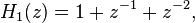
Transfer functions for the first (non-recursive) encoder are:

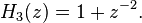
Transfer functions for the second (recursive) encoder are:
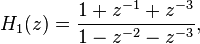

Define  by
by

where, for any rational function 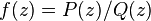 ,
,
 .
.
Then is the maximum of the polynomial degrees of the  , and the constraint length is defined as
  . For instance, in the first example the constraint length is 3, and in the second the constraint length is 4.
[edit] Trellis diagram
A convolutional encoder is a finite state machine. An encoder with n binary cells will have 2n states.
Imagine that the encoder (shown on Img.1, above) has '1' in the left memory cell (m0), and '0' in the right one (m-1). (m1 is not really a memory cell because it represents a current value). We will designate such a state as "10". According to an input bit the encoder at the next turn can convert either to the "01" state or the "11" state. One can see that not all transitions are possible (e.g., a decoder can't convert from "10" state to "00" or even stay in "10" state).
All possible transitions can be shown as below:

An actual encoded sequence can be represented as a path on this graph. One valid path is shown in red as an example.
This diagram gives us an idea about decoding: if a received sequence doesn't fit this graph, then it was received with errors, and we must choose the nearest correct (fitting the graph) sequence. The real decoding algorithms exploit this idea.
[edit] Free distance and error distribution
A free distance (d) is a minimal Hamming distance between different encoded sequences. A correcting capability (t) of a convolutional code is a number of errors that can be corrected by the code. It can be calculated as
Since a convolutional code doesn't use blocks, processing instead a continuous bitstream, the value of t applies to a quantity of errors located relatively near to each other. That is, multiple groups of t errors can usually be fixed when they are relatively far.
Free distance can be interpreted as a minimal length of an erroneous "burst" at the output of a convolutional decoder. The fact that errors appears as "bursts" should be accounted for when designing a concatenated code with an inner convolutional code. The popular solution for this problem is to interleave data before convolutional encoding, so that the outer block (usually Reed-Solomon) code can correct most of the errors.
[edit] Decoding convolutional codes
Several algorithms exist for decoding convolutional codes. For relatively small values of k, the Viterbi algorithm is universally used as it provides maximum likelihood performance and is highly parallelizable. Viterbi decoders are thus easy to implement in VLSI hardware and in software on CPUs with SIMD instruction sets.
Longer constraint length codes are more practically decoded with any of several sequential decoding algorithms, of which the Fano algorithm is the best known. Unlike Viterbi decoding, sequential decoding is not maximum likelihood but its complexity increases only slightly with constraint length, allowing the use of strong, long-constraint-length codes. Such codes were used in the Pioneer program of the early 1970s to Jupiter and Saturn, but gave way to shorter, Viterbi-decoded codes, usually concatenated with large Reed-Solomon error correction codes that steepen the overall bit-error-rate curve and produce extremely low residual undetected error rates.
Both Viterbi and sequential decoding algorithms return hard-decisions: the bits that form the most likely codeword. An approximate confidence measure can be added to each bit by use of the Soft output Viterbi algorithm. Maximum a posteriori (MAP) soft-decisions for each bit can be obtained by use of the BCJR algorithm.
[edit] Popular convolutional codes
An especially popular Viterbi-decoded convolutional code, used at least since the Voyager program has a constraint length k of 7 and a rate r of 1/2.
- Longer constraint lengths produce more powerful codes, but the complexity of the Viterbi algorithm increases exponentially with constraint lengths, limiting these more powerful codes to deep space missions where the extra performance is easily worth the increased decoder complexity.
- Mars Pathfinder, Mars Exploration Rover and the Cassini probe to Saturn use a k of 15 and a rate of 1/6; this code performs about 2 dB better than the simpler k=7 code at a cost of 256x in decoding complexity (compared to Voyager mission codes).
[edit] Punctured convolutional codes
Puncturing is a technique used to make a m/n rate code from a "basic" rate 1/2 code. It is reached by deletion of some bits in the encoder output. Bits are deleted according to puncturing matrix. The following puncturing matrices are the most frequently used:
| code rate | puncturing matrix | free distance (for NASA standard K=7 convolutional code) | ||||||||||||||
| 1/2 (No perf.) |
|
10 | ||||||||||||||
| 2/3 |
|
6 | ||||||||||||||
| 3/4 |
|
5 | ||||||||||||||
| 5/6 |
|
4 | ||||||||||||||
| 7/8 |
|
3 |
For example, if we want to make a code with rate 2/3 using the appropriate matrix from the above table, we should take a basic encoder output and transmit every second bit from the first branch and every bit from the second one. The specific order of transmission is defined by the respective communication standard.
Punctured convolutional codes are widely used in the satellite communications, for example, in INTELSAT systems and Digital Video Broadcasting.
Punctured convolutional codes are also called "perforated".
[edit] Turbo codes: replacing convolutional codes
Simple Viterbi-decoded convolutional codes are now giving way to turbo codes, a new class of iterated short convolutional codes that closely approach the theoretical limits imposed by Shannon's theorem with much less decoding complexity than the Viterbi algorithm on the long convolutional codes that would be required for the same performance. Turbo codes have not yet been concatenated with solid (low complexity) Reed-Solomon error correction codes.[citation needed] However, in the interest of planetary exploration this may someday be done.[citation needed]
[edit] See also
[edit] References
- This article contains material from the Federal Standard 1037C, which, as a work of the United States Government, is in the public domain.
[edit] External links
- Tutorial on Convolutional Coding and Decoding
- The on-line textbook: Information Theory, Inference, and Learning Algorithms, by David J.C. MacKay, discusses LDPC codes in Chapter 47.
- The Error Correcting Codes (ECC) Page

