Random variable

From Wikipedia, the free encyclopedia

In mathematics, random variables are used in the study of chance and probability. They were developed to assist in the analysis of games of chance, stochastic events, and the results of scientific experiments by capturing only the mathematical properties necessary to answer probabilistic questions. Further formalizations have firmly grounded the entity in the theoretical domains of mathematics by making use of measure theory.

Fortunately, the language and structure of random variables can be grasped at various levels of mathematical fluency. Set theory and calculus are fundamental.

Broadly, there are two types of random variables — discrete and continuous. Discrete random variables take on one of a set of specific values, each with some probability greater than zero. Continuous random variables can be realized with any of a range of values (e.g., a real number between zero and one), and so there are several ranges (e.g. 0 to one half) that have a probability greater than zero of occurring.

A random variable has either an associated probability distribution (discrete random variable) or probability density function (continuous random variable).

[edit] Intuitive definition

Intuitively, a random variable is thought of as a function mapping the sample space of a random process to the real numbers. A few examples will highlight this.

[edit] Examples

For a coin toss, the possible events are heads or tails. The number of heads appearing in one fair coin toss can be described using the following random variable:

$X = \begin{cases}1,& \text{if heads} ,\\ 0,& \text{if tails} .\end{cases}$

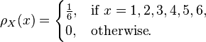
with probability mass function given by:

$\rho_X(x) = \begin{cases}\frac{1}{2},& \text{if }x=0,\\ \frac{1}{2},& \text{if }x=1,\\ 0,& \text{otherwise} .\end{cases}$

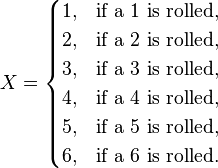
A random variable can also be used to describe the process of rolling a fair dice and the possible outcomes. The most obvious representation is to take the set {1, 2, 3, 4, 5, 6} as the sample space, defining the random variable X as the number rolled. In this case ,

$X = \begin{cases}1,& \text{if a 1 is rolled} ,\\ 2,& \text{if a 2 is rolled} ,\\ 3,& \text{if a 3 is rolled} ,\\ 4,& \text{if a 4 is rolled} ,\\ 5,& \text{if a 5 is rolled} ,\\ 6,& \text{if a 6 is rolled} .\end{cases}$

$\rho_X(x) = \begin{cases}\frac{1}{6},& \text{if }x=1,2,3,4,5,6,\\ 0,& \text{otherwise} .\end{cases}$

[edit] Formal definition

Let $(\Omega, \mathcal{F}, P)$ be a probability space and $(\mathcal{}Y, \Sigma)$ be a measurable space. Then a random variable X is formally defined as a measurable function $X: \Omega \rightarrow Y$ . An interpretation of this is that the preimage of the "well-behaved" subsets of Y (the elements of Σ) are events (elements of $\mathcal{F}$ ), and hence are assigned a probability by P.

[edit] Real-valued random variables

Typically, the measurable space is the measurable space over the real numbers. In this case, let $(\Omega, \mathcal{F}, P)$ be a probability space. Then, the function $X: \Omega \rightarrow \mathbb{R}$ is a real-valued random variable if

$\{ \omega : X(\omega) \le r \} \in \mathcal{F} \qquad \forall r \in \mathbb{R}$

[edit] Distribution functions of random variables

Associating a cumulative distribution function (CDF) with a random variable is a generalization of assigning a value to a variable. If the CDF is a (right continuous) Heaviside step function then the variable takes on the value at the jump with probability 1. In general, the CDF specifies the probability that the variable takes on particular values.

If a random variable $X: \Omega \to \mathbb{R}$ defined on the probability space $(\Omega, \mathcal{F}, P)$ is given, we can ask questions like "How likely is it that the value of $X$ is bigger than 2?". This is the same as the probability of the event $\{ s \in\Omega : X(s) > 2 \}$ which is often written as $P (X > 2)$ for short.

Recording all these probabilities of output ranges of a real-valued random variable X yields the probability distribution of X. The probability distribution "forgets" about the particular probability space used to define X and only records the probabilities of various values of X. Such a probability distribution can always be captured by its cumulative distribution function

$F_X(x) = \operatorname{P}(X \le x)$

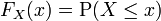
and sometimes also using a probability density function. In measure-theoretic terms, we use the random variable X to "push-forward" the measure P on Ω to a measure dF on R. The underlying probability space Ω is a technical device used to guarantee the existence of random variables, and sometimes to construct them. In practice, one often disposes of the space Ω altogether and just puts a measure on R that assigns measure 1 to the whole real line, i.e., one works with probability distributions instead of random variables.

[edit] Moments

The probability distribution of a random variable is often characterised by a small number of parameters, which also have a practical interpretation. For example, it is often enough to know what its "average value" is. This is captured by the mathematical concept of expected value of a random variable, denoted E[X]. In general, E[f(X)] is not equal to f(E[X]). Once the "average value" is known, one could then ask how far from this average value the values of X typically are, a question that is answered by the variance and standard deviation of a random variable.

Mathematically, this is known as the (generalised) problem of moments: for a given class of random variables X, find a collection {f_i} of functions such that the expectation values E[f_i(X)] fully characterize the distribution of the random variable X.

[edit] Functions of random variables

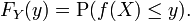
If we have a random variable X on Ω and a Borel measurable function f: R → R, then Y = f(X) will also be a random variable on Ω, since the composition of measurable functions is also measurable. (Warning: this is not true if f is Lebesgue measurable.) The same procedure that allowed one to go from a probability space (Ω, P) to (R, dF_X) can be used to obtain the distribution of Y. The cumulative distribution function of Y is

$F_Y(y) = \operatorname{P}(f(X) \le y).$

[edit] Example 1

Let X be a real-valued, continuous random variable and let Y = X².

$F_Y(y) = \operatorname{P}(X^2 \le y).$

If y < 0, then P(X² ≤ y) = 0, so

$F_Y(y) = 0\qquad\hbox{if}\quad y < 0.$

If y ≥ 0, then

$\operatorname{P}(X^2 \le y) = \operatorname{P}(|X| \le \sqrt{y}) = \operatorname{P}(-\sqrt{y} \le X \le \sqrt{y}),$

so

$F_Y(y) = F_X(\sqrt{y}) - F_X(-\sqrt{y})\qquad\hbox{if}\quad y \ge 0.$

[edit] Example 2

Suppose $\scriptstyle X$ is a random variable with a cumulative distribution

$F_{X}(x) = P(X \leq x) = \frac{1}{(1 + e^{-x})^{\theta}}$

where $\scriptstyle \theta > 0$ is a fixed parameter. Consider the random variable $\scriptstyle Y = \mathrm{log}(1 + e^{-X}).$ Then,

$F_{Y}(y) = P(Y \leq y) = P(\mathrm{log}(1 + e^{-X}) \leq y) = P(X > -\mathrm{log}(e^{y} - 1)).\,$

The last expression can be calculated in terms of the cumulative distribution of $X,$ so

$F_{Y}(y) = 1 - F_{X}(-\mathrm{log}(e^{y} - 1)) \,$

$= 1 - \frac{1}{(1 + e^{\mathrm{log}(e^{y} - 1)})^{\theta}}$

$= 1 - \frac{1}{(1 + e^{y} - 1)^{\theta}}$

$= 1 - e^{-y \theta}.\,$

[edit] Equivalence of random variables

There are several different senses in which random variables can be considered to be equivalent. Two random variables can be equal, equal almost surely, equal in mean, or equal in distribution.

In increasing order of strength, the precise definition of these notions of equivalence is given below.

[edit] Equality in distribution

Two random variables X and Y are equal in distribution if they have the same distribution functions:

$\operatorname{P}(X \le x) = \operatorname{P}(Y \le x)\quad\hbox{for all}\quad x.$

Two random variables having equal moment generating functions have the same distribution. This provides, for example, a useful method of checking equality of certain functions of i.i.d. random variables.

$d(X,Y)=\sup_x|\operatorname{P}(X \le x) - \operatorname{P}(Y \le x)|,$

which is the basis of the Kolmogorov-Smirnov test.

[edit] Equality in mean

Two random variables X and Y are equal in p-th mean if the pth moment of |X − Y| is zero, that is,

$\operatorname{E}(|X-Y|^p) = 0.$

As in the previous case, there is a related distance between the random variables, namely

$d_p(X, Y) = \operatorname{E}(|X-Y|^p).$

This is equivalent to the following:

[edit] Almost sure equality

Two random variables X and Y are equal almost surely if, and only if, the probability that they are different is zero:

$\operatorname{P}(X \neq Y) = 0.$

For all practical purposes in probability theory, this notion of equivalence is as strong as actual equality. It is associated to the following distance:

$d_\infty(X,Y)=\sup_\omega|X(\omega)-Y(\omega)|,$

where 'sup' in this case represents the essential supremum in the sense of measure theory.

[edit] Equality

Finally, the two random variables X and Y are equal if they are equal as functions on their probability space, that is,

$X(\omega)=Y(\omega)\qquad\hbox{for all}\quad\omega.$

[edit] Convergence

Much of mathematical statistics consists in proving convergence results for certain sequences of random variables; see for instance the law of large numbers and the central limit theorem.

There are various senses in which a sequence (X_n) of random variables can converge to a random variable X. These are explained in the article on convergence of random variables.

[edit] Literature

Kallenberg, O., Random Measures, 4th edition. Academic Press, New York, London; Akademie-Verlag, Berlin (1986). MR0854102 ISBN 0123949602
Kallenberg, O., Foundations of Modern Probability, 2nd edition. Springer-Verlag, New York, Berlin, Heidelberg (2001). ISBN 0-387-95313-2
Papoulis, Athanasios 1965 Probability, Random Variables, and Stochastic Processes. McGraw-Hill Kogakusha, Tokyo, 9th edition, ISBN 0-07-119981-0.

[edit] See also

Statistics portal

This article incorporates material from Random variable on PlanetMath, which is licensed under the GFDL.