Logistic regression
From Wikipedia, the free encyclopedia
In statistics, logistic regression (sometimes called the logistic model or logit model) is used for prediction of the probability of occurrence of an event by fitting data to a logistic curve. It is a generalized linear model used for binomial regression. Like many forms of regression analysis, it makes use of several predictor variables that may be either numerical or categorical. For example, the probability that a person has a heart attack within a specified time period might be predicted from knowledge of the person's age, sex and body mass index. Logistic regression is used extensively in the medical and social sciences as well as marketing applications such as prediction of a customer's propensity to purchase a product or cease a subscription.
Contents |
[edit] Lay explanation
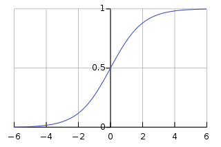
An explanation of logistic regression begins with an explanation of the logistic function:

A graph of the function is shown in figure 1. The "input" is z and the "output" is f(z). The logistic function is useful because it can take as an input any value from negative infinity to positive infinity, whereas the output is confined to values between 0 and 1. The variable z represents the exposure to some set of risk factors, while f(z) represents the probability of a particular outcome, given that set of risk factors. The variable z is a measure of the total contribution of all the risk factors used in the model and is known as the logit.
The variable z is usually defined as

where β0 is called the "intercept" and β1, β2, β3, and so on, are called the "regression coefficients" of x1, x2, x3 respectively. The intercept is the value of z when the value of all risk factors is zero (i.e., the value of z in someone with no risk factors). Each of the regression coefficients describes the size of the contribution of that risk factor. A positive regression coefficient means that that risk factor increases the probability of the outcome, while a negative regression coefficient means that risk factor decreases the probability of that outcome; a large regression coefficient means that the risk factor strongly influences the probability of that outcome; while a near-zero regression coefficient means that that risk factor has little influence on the probability of that outcome.
Logistic regression is a useful way of describing the relationship between one or more risk factors (e.g., age, sex, etc.) and an outcome such as death (which only takes two possible values: dead or not dead).
[edit] Example
The application of a logistic regression may be illustrated using a fictitious example of death from heart disease. This simplified model uses only three risk factors (age, sex, and blood cholesterol level) to predict the 10-year risk of death from heart disease. This is the model that we fit:
- β0 = − 5.0 (the intercept)
- β1 = + 2.0
- β2 = − 1.0
- β3 = + 1.2
- x1 = age in decades, less 5.0
- x2 = sex, where 0 is male and 1 is female
- x3 = cholesterol level, in mmol/L less 5.0
Which means the model is

In this model, increasing age is associated with an increasing risk of death from heart disease (z goes up by 2.0 for every 10 years over the age of 50), female sex is associated with a decreased risk of death from heart disease (z goes down by 1.0 if the patient is female), and increasing cholesterol is associated with an increasing risk of death (z goes up by 1.2 for each 1 mmol/L increase in cholesterol above 5mmol/L).
We wish to use this model to predict Mr Petrelli's risk of death from heart disease: he is 50 years old and his cholesterol level is 7.0 mmol/L. Mr Petrelli's risk of death is therefore

This means that by this model, Mr Petrelli's risk of dying from heart disease in the next 10 years is 0.07 (or 7%).
[edit] Formal mathematical specification
Logistic regression analyzes binomially distributed data of the form

where the numbers of Bernoulli trials ni are known and the probabilities of success pi are unknown. An example of this distribution is the fraction of seeds (pi) that germinate after ni are planted.
The model proposes for each trial (value of i) there is a set of explanatory variables that might inform the final probability. These explanatory variables can be thought of as being in a k vector Xi and the model then takes the form

The logits of the unknown binomial probabilities (i.e., the logarithms of the odds) are modelled as a linear function of the Xi.

Note that a particular element of Xi can be set to 1 for all i to yield an intercept in the model. The unknown parameters βj are usually estimated by maximum likelihood using a method common to all generalized linear models.
The interpretation of the βj parameter estimates is as the additive effect on the log odds ratio for a unit change in the jth explanatory variable. In the case of a dichotomous explanatory variable, for instance gender, eβ is the estimate of the odds ratio of having the outcome for, say, males compared with females.
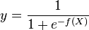
The model has an equivalent formulation

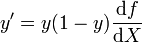
This functional form is commonly called a single-layer perceptron or single-layer artificial neural network. A single-layer neural network computes a continuous output instead of a step function. The derivative of pi with respect to X = x1...xk is computed from the general form:
where f(X) is an analytic function in X. With this choice, the single-layer network is identical to the logistic regression model. This function has a continuous derivative, which allows it to be used in backpropagation. This function is also preferred because its derivative is easily calculated:
[edit] Extensions
Extensions of the model cope with multi-category dependent variables and ordinal dependent variables, such as polytomous regression. Multi-class classification by logistic regression is known as multinomial logit modeling. An extension of the logistic model to sets of interdependent variables is the conditional random field.
[edit] See also
- Logistic function
- Sigmoid function
- Artificial neural network
- Data mining
- Linear discriminant analysis
- Perceptron
- Probit model
- Variable rules analysis
- Jarrow-Turnbull model
- Principle of maximum entropy
[edit] References
- Agresti, Alan. (2002). Categorical Data Analysis. New York: Wiley-Interscience. ISBN 0-471-36093-7.
- Amemiya, T. (1985). Advanced Econometrics. Harvard University Press. ISBN 0-674-00560-0.
- Balakrishnan, N. (1991). Handbook of the Logistic Distribution. Marcel Dekker, Inc.. ISBN 978-0824785871.
- Greene, William H. (2003). Econometric Analysis, fifth edition. Prentice Hall. ISBN 0-13-066189-9.
- Hilbe, Joseph M. (2009). Logistic Regression Models. Chapman & Hall/CRC Press. ISBN 978-1-4200-7575-5.
- Hosmer, David W.; Stanley Lemeshow (2000). Applied Logistic Regression, 2nd ed.. New York; Chichester, Wiley. ISBN 0-471-35632-8.
|
|||||||||||||||||||||||||||||||||||||||||||||||||||||||||

