ciencia classroomresource elecromagnetism electrical electromagnetic electromagnetism eletromagnetismo em engineering equations erik fourier_optics_material group henry ligninger magnetism math mathematics maxwell maxwell's maxwells maxwellsequations my_reserve_shelf physics science simulation solid 4

My tags:

From Wikipedia, the free encyclopedia

Electromagnetism

Electricity · Magnetism Electrostatics Electric charge · Coulomb's law · Electric field · Electric flux · Gauss's law · Electric potential · Electrostatic induction · Electric dipole moment · Magnetostatics Ampère’s law · Electric current · Magnetic field · Magnetic flux · Biot–Savart law · Magnetic dipole moment · Gauss’s law for magnetism · Electrodynamics Free space · Lorentz force law · EMF · Electromagnetic induction · Faraday’s law · Displacement current · Maxwell’s equations · EM field · Electromagnetic radiation · Liénard-Wiechert Potential · Maxwell tensor · Eddy current · Electrical Network Electrical conduction · Electrical resistance · Capacitance · Inductance · Impedance · Resonant cavities · Waveguides · Covariant formulation Electromagnetic tensor · EM Stress-energy tensor · Four-current · Four-potential · Scientists Ampère · Coulomb · Faraday · Heaviside · Henry · Hertz · Lorentz · Maxwell · Tesla · Weber ·

This box: view • talk • edit

In electromagnetism, Maxwell's equations are a set of four partial differential equations that describe the properties of the electric and magnetic fields and relate them to their sources, charge density and current density. These equations are used to show that light is an electromagnetic wave. Individually, the equations are known as Gauss's law, Gauss's law for magnetism, Faraday's law of induction, and Ampère's law with Maxwell's correction.

These four equations, together with the Lorentz force law are the complete set of laws of classical electromagnetism. The Lorentz force law itself was actually derived by Maxwell under the name of "Equation for Electromotive Force" and was one of an earlier set of eight Maxwell's equations.

Contents 1 Conceptual description 2 General formulation 2.1 Table 1: Formulation in terms of free charge and current 2.2 Table 2: Formulation in terms of total charge and current 2.3 Table 3: Definitions and units 3 History 3.1 The term Maxwell's equations 3.2 Maxwell's On Physical Lines of Force (1861) 3.3 Maxwell's A Dynamical Theory of the Electromagnetic Field (1865) 4 Details and special cases 4.1 Bound charge and current 4.1.1 Proof that the two general formulations are equivalent 4.2 Constitutive relations 4.2.1 Case without magnetic or dielectric materials 4.2.2 Case of linear materials 4.2.3 General case 4.2.4 Maxwell's equations in terms of E and B for linear materials 4.3 In vacuum 4.4 With magnetic monopoles 5 Materials and dynamics 5.1 Boundary conditions 6 CGS units 7 Special relativity 7.1 Historical developments 7.2 Covariant formulation of Maxwell's equations 8 Potentials 9 Differential forms 9.1 Conceptual insight from this formulation 10 Classical electrodynamics as the curvature of a line bundle 11 Curved spacetime 11.1 Traditional formulation 11.2 Formulation in terms of differential forms 12 See also 13 References 14 Further reading 14.1 Journal articles 14.2 University level textbooks 14.2.1 Undergraduate 14.2.2 Graduate 14.2.3 Older classics 14.2.4 Computational techniques 15 External links 15.1 Modern treatments 15.2 Historical 15.3 Other

[edit] Conceptual description

This section will conceptually describe each of the four Maxwell's equations, and also how they link together to explain the origin of electromagnetic radiation such as light. The exact equations can be found in the subsequent section.

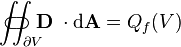
• Gauss's law relates electric charge contained within a closed surface (Gaussian surface) to the surrounding electric field. It describes with mathematical clarity how the divergence of an electrical field is affected by charges (electric field lines diverge from positive charges and are drawn towards negative charges). It also states that the total electric flux through a Gaussian surface is unrelated to the shape and size of that surface.

• Gauss's law for magnetism states that the total magnetic flux through a Gaussian Surface is zero. This is due to the fact that real world magnetic charges come in pairs (referred to as dipoles) and the two charges create opposite magnetic field divergences; which cancel each other out. The theoretical single magnetic charge is referred to as a magnetic monopole. Gauss's Law for Magnetism is also used to state mathematically that magnetic monopoles do not exist.

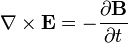
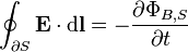
• Faraday's law of induction describes how a changing magnetic field can create an electric field. This is, for example, the operating principle behind many electric generators: Mechanical force (such as the force of water falling through a hydroelectric dam) spins a huge magnet, and the changing magnetic field creates an electric field which drives electricity through the power grid.

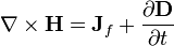
• Ampère's law with Maxwell's correction states that magnetic fields can be generated in two ways: By electrical current (this was the original "Ampère's law") and by changing electric fields. The idea that a magnetic field can be induced by a changing electric field follows from the modern concept of displacement current which was introduced to maintain the solenoidal nature of Ampère's law in a vacuum capacitor circuit. This modern displacement current concept has the same mathematical form as Maxwell's original displacement current. Maxwell's original displacement current applies to polarization current in a dielectric medium and it sits adjacent to the modern displacement current in Ampère's law.

Maxwell's correction to Ampère's law was particularly important: In 1864 Maxwell derived the electromagnetic wave equation by linking the displacement current to the time-varying electric field that is associated with electromagnetic induction. This is described in A Dynamical Theory of the Electromagnetic Field, where he commented:

The agreement of the results seems to show that light and magnetism are affections of the same substance, and that light is an electromagnetic disturbance propagated through the field according to electromagnetic laws.^[1]

The modern extension to displacement current applies in the pure vacuum. This is interpreted as meaning that a changing electric field can produce a magnetic field, and vice-versa. Under this modern interpretation, it follows that, even with no electric charges or currents present, it's possible to have stable, self-perpetuating waves of oscillating electric and magnetic fields, with each field driving the other. The physical parameters of transverse elasticity and density, which Maxwell used to calculate the speed of these electromagnetic waves have now given way to two easily-measurable physical constants called the electric constant and the magnetic constant).

The speed calculated for electromagnetic radiation exactly matches the speed of light; indeed, light is one form of electromagnetic radiation (as are X-rays, radio waves, and others). In this way, Maxwell unified the hitherto separate fields of electromagnetism and optics.

[edit] General formulation

The equations in this section are given in SI units. Unlike the equations of mechanics (for example), Maxwell's equations are not unchanged in other unit systems. Though the general form remains the same, various definitions get changed and different constants appear at different places. Other than SI (used in engineering), the units commonly used are Gaussian units (based on the cgs system and considered to have some theoretical advantages over SI^[2]), Lorentz-Heaviside units (used mainly in particle physics) and Planck units (used in theoretical physics). See below for CGS-Gaussian units.

Two equivalent, general formulations of Maxwell's equations follow. The first separates bound charge and bound current (which arise in the context of dielectric and/or magnetized materials) from free charge and free current (the more conventional type of charge and current). This separation is useful for calculations involving dielectric or magnetized materials. The second formulation treats all charge equally, combining free and bound charge into total charge (and likewise with current). This is the more fundamental or microscopic point of view, and is particularly useful when no dielectric or magnetic material is present. More details, and a proof that these two formulations are mathematically equivalent, are given in section 3.

Symbols in bold represent vector quantities, whereas symbols in italics represent scalar quantities. The definitions of terms used in the two tables of equations are given in another table immediately following.

[edit] Table 1: Formulation in terms of free charge and current

Name	Differential form	Integral form
Gauss's law:
Gauss's law for magnetism:
Maxwell-Faraday equation (Faraday's law of induction):
Ampère's circuital law (with Maxwell's correction):

Here V is a three-dimensional volume, S a two-dimensional oriented surface; Q(V) the electrical charge (free rsp. total) contained in V, and I_S the electrical current flowing through S. is the flux of the magnetic field flowing through S.

[edit] Table 2: Formulation in terms of total charge and current

For the total quantities one has an analogous table;

Name	Differential form	Integral form
Gauss's law:
Gauss's law for magnetism:
Maxwell-Faraday equation (Faraday's law of induction):
Ampère's circuital law (with Maxwell's correction):

The following table provides the meaning of each symbol and the SI unit of measure:

[edit] Table 3: Definitions and units

Symbol	Meaning (first term is the most common)	SI Unit of Measure
	electric field	volt per meter or, equivalently, newton per coulomb
	magnetic field also called the magnetic induction also called the magnetic field density also called the magnetic flux density	tesla, or equivalently, weber per square meter volt•second per square meter
	electric displacement field also called the electric flux density	coulombs per square meter or, equivalently, newton per volt-meter
	magnetizing field also called auxiliary magnetic field also called magnetic field intensity also called magnetic field	ampere per meter
	the divergence operator	per meter (factor contributed by applying either operator)
	the curl operator
	partial derivative with respect to time	per second (factor contributed by applying the operator)
	differential vector element of surface area A, with infinitesimally small magnitude and direction normal to surface S	square meters
	differential vector element of path length tangential to the path/curve	meters
	permittivity of free space, officially the electric constant, a universal constant	farads per meter
	permeability of free space, officially the magnetic constant, a universal constant	henries per meter, or Newtons per ampere squared
	free charge density (not including bound charge)	coulombs per cubic meter
	total charge density (including both free and bound charge)	coulombs per cubic meter
	free current density (not including bound current)	amperes per square meter
	total current density (including both free and bound current)	amperes per square meter
	net unbalanced free electric charge in the interior of an arbitrary closed surface (not including bound charge)	coulombs
	net unbalanced electric charge in the interior of an arbitrary closed surface (including both free and bound charge)	coulombs
	line integral of the electric field along the boundary ∂S (therefore necessarily a closed curve) of the surface S	joules per coulomb
	line integral of the magnetic field over the closed boundary ∂S of the surface S	tesla-meters
	the flux of the electric field through any closed surface	joule-meter per coulomb
	the flux of the magnetic field through any closed surface	tesla meters-squared or webers
	magnetic flux through any surface S (not necessarily closed)	webers or equivalently, volt-seconds
	electric flux through any surface S, not necessarily closed	joule-meters per coulomb
	flux of electric displacement field through any surface S, not necessarily closed	coulombs
	net free electrical current passing through the surface S (not including bound current)	amperes
	net electrical current passing through the surface S (including both free and bound current)	amperes

Maxwell's equations are generally applied to macroscopic averages of the fields, which vary wildly on a microscopic scale in the vicinity of individual atoms (where they undergo quantum mechanical effects as well). It is only in this averaged sense that one can define quantities such as the permittivity and permeability of a material. At the microscopic level, Maxwell's equations, ignoring quantum effects, describe fields, charges and currents in free space — but at this level of detail one must include all charges, even those at an atomic level, generally an intractable problem.

[edit] History

Although James Clerk Maxwell was not the originator of these equations in modern notation, he nevertheless derived three of them again independently in conjunction with his molecular vortex model of Faraday's "lines of force", along with the full version of Faraday's law of induction. In doing so he made an important addition to Ampère's circuital law.

Nevertheless all four of what are now described as Maxwell's equations can be found in recognisable form in vol. 2 of Maxwell's "A Treatise on Electricity & Magnetism", published in 1873, in Chapter IX, entitled "General Equations of the Electromagnetic Field". This book by Maxwell pre-dates Heaviside's and other publications.

Maxwell also developed Faraday's law of induction into another equation, which used to be listed as a 'Maxwell's equation' but is nowadays known as the Lorentz force law.^[3]

[edit] The term Maxwell's equations

Controversy has always surrounded the term Maxwell's equations concerning the extent to which Maxwell himself was involved in these equations. The term Maxwell's equations nowadays applies to a set of four equations that were grouped together as a distinct set in 1884 by Oliver Heaviside, in conjunction with Willard Gibbs. However it is perhaps difficult to see the basis of a controversy: if Heaviside and Gibbs selected and highlighted four of Maxwell's equations, that does not imply a change of 'ownership'. Thus the 'controversy' appears somewhat artificial.

The importance of Maxwell's role in these equations lies in the correction he made to Ampère's circuital law in his 1861 paper On Physical Lines of Force. He added the displacement current term to Ampère's circuital law and this enabled him to derive the electromagnetic wave equation in his later 1865 paper A Dynamical Theory of the Electromagnetic Field and demonstrate the fact that light is an electromagnetic wave. This fact was then later confirmed experimentally by Heinrich Hertz in 1887.

The reason that these equations are called Maxwell's equations is sometimes disputed. Some say that these equations were originally called the Hertz-Heaviside equations but that Einstein for whatever reason later referred to them as the Maxwell-Hertz equations. See pages 110-112 of Nahin's book^[4][5]

The equations are based on the works of James Clerk Maxwell, and were published by Maxwell in his 'A Treatise on Electricity & Magnetism' of 1873, and Heaviside made no secret of the fact that he was working from Maxwell's papers. Heaviside selected a symmetrical set of equations that were crucial as regards deriving the telegrapher's equations. The net result was a set of four equations, all of which had appeared in Maxwell's previous publications, in particular Maxwell's 1861 paper On Physical Lines of Force and 1865 paper A Dynamical Theory of the Electromagnetic Field. The fourth was a partial time derivative version of Faraday's law of induction that doesn't include motionally induced EMF.^[6]

Of Heaviside's equations, the most important in deriving the telegrapher's equations was the version of Ampère's circuital law that had been amended by Maxwell in this 1861 paper to include what is termed the displacement current.

[edit] Maxwell's On Physical Lines of Force (1861)

(Alternate source.)

Three of Heaviside's four equations appeared throughout Maxwell's 1861 paper On Physical Lines of Force, but all appear in Maxwell's 'Treatise':

(i) At equation (56) of Maxwell's 1861 paper we see .

(ii) At equation (112) we see Ampère's circuital law with Maxwell's correction. It is this correction called displacement current which is the most significant aspect of Maxwell's work in electromagnetism as it enabled him to later derive the electromagnetic wave equation in his 1865 paper A Dynamical Theory of the Electromagnetic Field, and hence show that light is an electromagnetic wave. It is therefore this aspect of Maxwell's work which gives Heaviside's equations their full significance. (Interestingly, Kirchhoff derived the telegrapher's equations in 1857 without using displacement current. But he did use Poisson's equation and the equation of continuity which are the mathematical ingredients of the displacement current. Nevertheless, Kirchhoff believed his equations to be applicable only inside an electric wire and so he is not credited with having discovered that light is an electromagnetic wave).

(iii) At equation (115) we see Gauss's law.

(iv) Heaviside's fourth equation introduced a restricted partial time derivative version of Faraday's law of induction. (A full version of Faraday's law of induction had appeared at equation (54) of Maxwell's 1861 paper). It is important however to note that Heaviside's partial time derivative notation, as opposed to the total time derivative notation used by Maxwell at equations (54), resulted in the loss of the v × B term that appeared in Maxwell's equation (77). Nowadays, the v × B term appears in the force law F = q ( E + v × B ) which sits adjacent to Maxwell's equations and bears the name Lorentz force. The Lorentz Force corresponds in effect to Maxwell's equation (77), but it appeared in this paper when Lorentz was still a young boy.

[edit] Maxwell's A Dynamical Theory of the Electromagnetic Field (1865)

Confusion over the term "Maxwell's equations" is exacerbated because it is also sometimes used for a set of eight equations that appeared in Part III of Maxwell's 1865 paper A Dynamical Theory of the Electromagnetic Field, entitled "General Equations of the Electromagnetic Field",^[7] a confusion compounded by the writing of six of those eight equations as three separate equations (one for each of the Cartesian axes), resulting in twenty equations in twenty unknowns. (As noted above, this terminology is not common: Modern references to the term "Maxwell's equations" usually refer to the Heaviside restatements.)

These original eight equations are nearly identical to the Heaviside versions in substance, but they have some superficial differences. In fact, only one of the Heaviside versions is completely unchanged from these original equations, and that is Gauss's law (Maxwell's equation G below). Another of Heaviside's four equations is an amalgamation of Maxwell's law of total currents (equation A below) with Ampère's circuital law (equation C below). This amalgamation, which Maxwell himself originally made at equation (112) in his 1861 paper "On Physical Lines of Force" (see above), is the one that modifies Ampère's circuital law to include Maxwell's displacement current.

The eight original Maxwell's equations can be written in modern vector notation as follows:

(A) The law of total currents

(B) The equation of magnetic force

(C) Ampère's circuital law

(D) Electromotive force created by convection, induction, and by static electricity. (This is in effect the Lorentz force)

(E) The electric elasticity equation

(F) Ohm's law

(G) Gauss's law

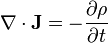
(H) Equation of continuity

Notation

is the magnetizing field, which Maxwell called the "magnetic intensity".

is the electric current density (with being the total current including displacement current).

is the displacement field (called the "electric displacement" by Maxwell).

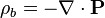
ρ is the free charge density (called the "quantity of free electricity" by Maxwell).

is the magnetic vector potential (called the "angular impulse" by Maxwell).

is called the "electromotive force" by Maxwell. The term electromotive force is nowadays used for voltage, but it is clear from the context that Maxwell's meaning corresponded more to the modern term electric field.

Φ is the electric potential (which Maxwell also called "electric potential").

σ is the electrical conductivity (Maxwell called the inverse of conductivity the "specific resistance", what is now called the resistivity).

It is interesting to note the term that appears in equation D. Equation D is therefore effectively the Lorentz force, similarly to equation (77) of his 1861 paper (see above).

When Maxwell derives the electromagnetic wave equation in his 1865 paper, he uses equation D to cater for electromagnetic induction rather than Faraday's law of induction which is used in modern textbooks. (Faraday's law itself does not appear among his equations.) However, Maxwell drops the term from equation D when he is deriving the electromagnetic wave equation, as he considers the situation only from the rest frame.

[edit] Details and special cases

[edit] Bound charge and current

If an electric field is applied to a dielectric material, each of the molecules responds by forming a microscopic dipole -- its atomic nucleus will move a tiny distance in the direction of the field, while its electrons will move a tiny distance in the opposite direction. This is called polarization of the material. The distribution of charge that results from these tiny movements turn out to be identical to having a layer of positive charge on one side of the material, and a layer of negative charge on the other side -- a macroscopic separation of charge, even though all of the charges involved are "bound" to a single molecule. This is called bound charge. Likewise, in a magnetized material, there is effectively a "bound current" circulating around the material, despite the fact that no individual charge is travelling a distance larger than a single molecule.

[edit] Proof that the two general formulations are equivalent

In this section, a simple proof is outlined which shows that the two alternate general formulations of Maxwell's equations given in Section 1 are mathematically equivalent.

The relation between polarization, magnetization, bound charge, and bound current is as follows:

where P and M are polarization and magnetization, and ρ_b and J_b are bound charge and current, respectively. Plugging in these relations, it can be easily demonstrated that the two formulations of Maxwell's equations given in Section 1 are precisely equivalent.

[edit] Constitutive relations

In order to apply Maxwell's equations (the formulation in terms of free charge and current, and D and H), it is necessary to specify the relations between D and E, and H and B. These are called constitutive relations, and correspond physically to specifying the response of bound charge and current to the field, or equivalently, how much polarization and magnetization a material acquires in the presence of electromagnetic fields.

[edit] Case without magnetic or dielectric materials

In the absence of magnetic or dielectric materials, the relations are simple:

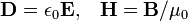
where ε₀ and μ₀ are two universal constants, called the permittivity of free space and permeability of free space, respectively.

[edit] Case of linear materials

In a "linear", isotropic, nondispersive, uniform material, the relations are also straightforward:

where ε and μ are constants (which depend on the material), called the permittivity and permeability, respectively, of the material.

[edit] General case

For real-world materials, the constitutive relations are not simple proportionalities, except approximately. The relations can usually still be written:

but ε and μ are not, in general, simple constants, but rather functions. For example, ε and μ can depend upon:

• The strength of the fields (the case of nonlinearity, which occurs when ε and μ are functions of E and B; see, for example, Kerr and Pockels effects),
• The direction of the fields (the case of anisotropy, birefringence, or dichroism; which occurs when ε and μ are second-rank tensors),
• The frequency with which the fields vary (the case of dispersion, which occurs when ε and μ are functions of frequency; see, for example, Kramers–Kronig relations).

If further there are dependencies on:

• The position inside the material (the case of a nonuniform material, which occurs when the response of the material varies from point to point within the material, an effect called spatial dispersion; for example in a domained structure, heterostructure or a liquid crystal, or principally in any bounded medium),
• The history of the fields (the case of hysteresis, which occurs when the repsonse of the material is a function of both present and past values of the fields),

then the constitutive relations take a more complicated form:^[8][9]

,

in which the permittivity and permeability functions are replaced by integrals over the more general electric and magnetic susceptibilities.

[edit] Maxwell's equations in terms of E and B for linear materials

Substituting in the constitutive relations above, Maxwell's equations in a linear material (differential form only) are:

These are formally identical to the general formulation in terms of E and B (given above), except that the permittivity of free space was replaced with the permittivity of the material (see also displacement field, electric susceptibility and polarization density), the permeability of free space was replaced with the permeability of the material (see also magnetization, magnetic susceptibility and magnetic field), and only free charges and currents are included (instead of all charges and currents).

[edit] In vacuum

Starting with the equations appropriate in the case without dielectric or magnetic materials, and assuming that there is no current or electric charge present in the vacuum, we obtain the Maxwell equations in free space:

These equations have a solution in terms of traveling sinusoidal plane waves, with the electric and magnetic field directions orthogonal to one another and the direction of travel, and with the two fields in phase, traveling at the speed^[10]

In fact, Maxwell's equations explains specifically how these waves can physically propagate through space. The changing magnetic field creates a changing electric field through Faraday's law. That electric field, in turn, creates a changing magnetic field through Maxwell's correction to Ampère's law. This perpetual cycle allows these waves, known as electromagnetic radiation, to move through space, always at velocity c.

Maxwell discovered that this quantity c equals the speed of light in vacuum (known from early experiments), and concluded (correctly) that light is a form of electromagnetic radiation.

[edit] With magnetic monopoles

Maxwell's equations of electromagnetism relate the electric and magnetic fields to the motions of electric charges. The standard form of the equations provide for an electric charge, but posit no magnetic charge (in accordance with the fact that magnetic charge has never been seen and may not exist). Except for this, the equations are symmetric under interchange of electric and magnetic field. In fact, symmetric equations can be written when all charges are zero, and this is how the wave equation is derived (see immediately above).

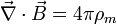
Fully symmetric equations can also be written if one allows for the possibility of "magnetic charges" analogous to electric charges.^[11] With the inclusion of a variable for these magnetic charges, say , there will also be "magnetic current" variable in the equations, . The extended Maxwell's equations, simplified by nondimensionalization via Planck units, are as follows:

Name	Without magnetic monopoles	With magnetic monopoles (hypothetical)
Gauss's law:
Gauss's law for magnetism:
Maxwell-Faraday equation (Faraday's law of induction):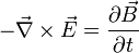
Ampère's law (with Maxwell's extension):
Note: the Bivector notation embodies the sign swap, and these four equations can be written as only one equation.

If magnetic charges do not exist, or if they exist but where they are not present in a region, then the new variables are zero, and the symmetric equations reduce to the conventional equations of electromagnetism such as . Classically, the question is "Why does the magnetic charge always seem to be zero?"

[edit] Materials and dynamics

The fields in Maxwell's equations are generated by charges and currents. Conversely, the charges and currents are affected by the fields through the Lorentz force equation:

where q is the charge on the particle and v is the particle velocity. (It also should be remembered that the Lorentz force is not the only force exerted upon charged bodies, which also may be subject to gravitational, nuclear, etc. forces.) Therefore, in both classical and quantum physics, the precise dynamics of a system form a set of coupled differential equations, which are almost always too complicated to be solved exactly, even at the level of statistical mechanics.^[12] This remark applies to not only the dynamics of free charges and currents (which enter Maxwell's equations directly), but also the dynamics of bound charges and currents, which enter Maxwell's equations through the constitutive equations, as described next.

Commonly, real materials are approximated as "continuum" media with bulk properties such as the refractive index, permittivity, permeability, conductivity, and/or various susceptibilities. These lead to the macroscopic Maxwell's equations, which are written (as given above) in terms of free charge/current densities and D, H, E, and B ( rather than E and B alone ) along with the constitutive equations relating these fields. For example, although a real material consists of atoms whose electronic charge densities can be individually polarized by an applied field, for most purposes behavior at the atomic scale is not relevant and the material is approximated by an overall polarization density related to the applied field by an electric susceptibility.

Continuum approximations of atomic-scale inhomogeneities cannot be determined from Maxwell's equations alone. but require some type of quantum mechanical analysis such as quantum field theory as applied to condensed matter physics. See, for example, density functional theory, Green–Kubo relations and Green's function (many-body theory). Various approximate transport equations have evolved, for example, the Boltzmann equation or the Fokker–Planck equation or the Navier-Stokes equations. Some examples where these equations are applied are magnetohydrodynamics, fluid dynamics, electrohydrodynamics, superconductivity, plasma modeling. An entire physical apparatus for dealing with these matters has developed. A different set of homogenization methods (evolving from a tradition in treating materials such as conglomerates and laminates) are based upon approximation of an inhomogeneous material by a homogeneous effective medium^[13][14] (valid for excitations with wavelengths much larger than the scale of the inhomogeneity).^{[15][16][17][18]}

Theoretical results have their place, but often require fitting to experiment. Continuum-approximation properties of many real materials rely upon measurement,^[19] for example, ellipsometry measurements.

In practice, some materials properties have a negligible impact in particular circumstances, permitting neglect of small effects. For example: optical nonlinearities can be neglected for low field strengths; material dispersion is unimportant where frequency is limited to a narrow bandwidth; material absorption can be neglected for wavelengths where a material is transparent; and metals with finite conductivity often are approximated at microwave or longer wavelengths as perfect metals with infinite conductivity (forming hard barriers with zero skin depth of field penetration).

And, of course, some situations demand that Maxwell's equations and the Lorentz force be combined with other forces that are not electromagnetic. An obvious example is gravity. A more subtle example, which applies where electrical forces are weakened due to charge balance in a solid or a molecule, is the Casimir force from quantum electrodynamics.^[20]

The connection of Maxwell's equations to the rest of the physical world is via the fundamental sources of charges and currents and the forces on them, and also by the properties of physical materials.

[edit] Boundary conditions

Although Maxwell's equations apply throughout space and time, practical problems are finite and solutions to Maxwell's equations inside the solution region are joined to the remainder of the universe through boundary conditions^[21][22][23] and started in time using initial conditions.^[24] In some cases, like waveguides or cavity resonators, the solution region is largely isolated from the universe, for example, by metallic walls, and boundary conditions at the walls define the fields with influence of the outside world confined to the input/output ends of the structure.^[25] In other cases, the universe at large sometimes is approximated by an artificial absorbing boundary,^[26][27][28] or, for example for radiating antennas or communication satellites, these boundary conditions can take the form of asymptotic limits imposed upon the solution.^[29] In addition, for example in an optical fiber or thin-film optics, the solution region often is broken up into subregions with their own simplified properties, and the solutions in each subregion must be joined to each other across the subregion interfaces using boundary conditions.^[30][31][32] Following are some links of a general nature concerning boundary value problems: Examples of boundary value problems, Sturm-Liouville theory, Dirichlet boundary condition, Neumann boundary condition, mixed boundary condition, Cauchy boundary condition, Sommerfeld radiation condition. Needless to say, one must choose the boundary conditions appropriate to the problem being solved. See also Kempel^[33] and the extraordinary book by Friedman.^[34]

[edit] CGS units

The above equations are given in the International System of Units, or SI for short. In a related unit system, called cgs (short for centimeter-gram-second), the equations take the following form:

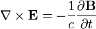
where c is the speed of light in a vacuum. For the electromagnetic field in a vacuum, the equations become:

In this system of units the relation between displacement field, electric field and polarization density is:

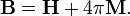
And likewise the relation between magnetic induction, magnetic field and total magnetization is:

In the linear approximation, the electric susceptibility and magnetic susceptibility can be defined so that:

,    

(Note that although the susceptibilities are dimensionless numbers in both cgs and SI, they have different values in the two unit systems, by a factor of 4π.) The permittivity and permeability are:

,    

so that

,    

In vacuum, one has the simple relations , D=E, and B=H.

The force exerted upon a charged particle by the electric field and magnetic field is given by the Lorentz force equation:

where is the charge on the particle and is the particle velocity. This is slightly different from the SI-unit expression above. For example, here the magnetic field has the same units as the electric field .

[edit] Special relativity

Maxwell's equations have a close relation to special relativity: Not only were Maxwell's equations a crucial part of the historical development of special relativity, but also, special relativity has motivated a compact mathematical formulation of Maxwell's equations, in terms of covariant tensors.

[edit] Historical developments

Maxwell's electromagnetic wave equation only applied in what he believed to be the rest frame of the luminiferous medium because he didn't use the vXB term of his equation (D) when he derived it. Maxwell's idea of the luminiferous medium was that it comprised of aethereal vortices aligned solenoidally along their rotation axes.

The American scientist A.A. Michelson set out to determine the velocity of the earth through the luminiferous medium aether using a light wave interferometer that he had invented. When the Michelson-Morley experiment was conducted by Edward Morley and Albert Abraham Michelson in 1887, it produced a null result for the change of the velocity of light due to the Earth's motion through the hypothesized aether. This null result was in line with the theory that was proposed in 1845 by George Stokes which suggested that the aether was entrained with the Earth's orbital motion.

Hendrik Lorentz objected to Stokes' aether drag model and along with George FitzGerald and Joseph Larmor, he suggested another approach. Both Larmor (1897) and Lorentz (1899, 1904) derived the Lorentz transformation (so named by Henri Poincaré) as one under which Maxwell's equations were invariant. Poincaré (1900) analyzed the coordination of moving clocks by exchanging light signals. He also established mathematically the group property of the Lorentz transformation (Poincaré 1905).

This culminated in Albert Einstein's revolutionary theory of special relativity, which postulated the absence of any absolute rest frame, dismissed the aether as unnecessary (a bold idea, which did not come to Lorentz nor to Poincaré), and established the invariance of Maxwell's equations in all inertial frames of reference, in contrast to the famous Newtonian equations for classical mechanics. But the transformations between two different inertial frames had to correspond to Lorentz' equations and not - as formerly believed - to those of Galileo (called Galilean transformations).^[35] Indeed, Maxwell's equations played a key role in Einstein's famous paper on special relativity; for example, in the opening paragraph of the paper, he motivated his theory by noting that a description of a conductor moving with respect to a magnet must generate a consistent set of fields irrespective of whether the force is calculated in the rest frame of the magnet or that of the conductor.^[36]

General relativity has also had a close relationship with Maxwell's equations. For example, Kaluza and Klein showed in the 1920s that Maxwell's equations can be derived by extending general relativity into five dimensions. This strategy of using higher dimensions to unify different forces continues to be an active area of research in particle physics.

[edit] Covariant formulation of Maxwell's equations

In special relativity, in order to more clearly express the fact that Maxwell's equations in vacuum take the same form in any inertial coordinate system, Maxwell's equations are written in terms of four-vectors and tensors in the "manifestly covariant" form. The purely spatial components of the following are in SI units.

One ingredient in this formulation is the electromagnetic tensor, a rank-2 covariant antisymmetric tensor combining the electric and magnetic fields:

and the result of raising its indices

The other ingredient is the four-current: where ρ is the charge density and J is the current density.

With these ingredients, Maxwell's equations can be written:

and

The first tensor equation is an expression of the two inhomogeneous Maxwell's equations, Gauss's law and Ampere's law with Maxwell's correction. The second equation is an expression of the two homogeneous equations, Faraday's law of induction and Gauss's law for magnetism. The second equation is equivalent to

where is the contravariant version of the Levi-Civita symbol, and

is the 4-gradient. In the tensor equations above, repeated indices are summed over according to Einstein summation convention. We have displayed the results in several common notations. Upper and lower components of a vector, v^α and v_α respectively, are interchanged with the fundamental tensor g, e.g., g=η=diag(-1,+1,+1,+1).

Alternative covariant presentations of Maxwell's equations also exist, for example in terms of the four-potential; see Covariant formulation of classical electromagnetism for details.

[edit] Potentials

Maxwell's equations can be written in an alternative form, involving the electric potential (also called scalar potential) and magnetic potential (also called vector potential), as follows.^[9] (The following equations are valid in the absence of dielectric and magnetic materials; or if such materials are present, they are valid as long as bound charge and bound current are included in the total charge and current densities.)

First, Gauss's law for magnetism states:

By Helmholtz's theorem, B can be written in terms of a vector field A, called the magnetic potential:

Second, plugging this into Faraday's law, we get:

By Helmholtz's theorem, the quantity in parentheses can be written in terms of a scalar function Φ, called the electric potential:

Combining these with the remaining two Maxwell's equations yields the four relations:

These equations, taken together, are as powerful and complete as Maxwell's equations. Moreover, the problem has been reduced somewhat, as the electric and magnetic fields each have three components which need to be solved for (six components altogether), while the electric and magnetic potentials have only four components altogether. On the other hand, these equations appear more complicated than Maxwell's equations using just the electric and magnetic fields.

In fact, these equations can be simplified a good deal by taking advantage of gauge freedom—i.e., the fact that there are many different choices of A and Φ consistent with a given E and B. For more information, see the article gauge freedom.

[edit] Differential forms

In free space, where ε = ε₀ and μ = μ₀ are constant everywhere, Maxwell's equations simplify considerably once the language of differential geometry and differential forms is used. In what follows, cgs units, not SI units are used, however. The electric and magnetic fields are now jointly described by a 2-form F in a 4-dimensional spacetime manifold. Maxwell's equations then reduce to the Bianchi identity

where d denotes the exterior derivative — a natural coordinate and metric independent differential operator acting on forms — and the source equation

where the (dual) Hodge star operator * is a linear transformation from the space of 2-forms to the space of (4-2)-forms defined by the metric in Minkowski space (in four dimensions even by any metric conformal to this metric), and the fields are in natural units where 1 / 4πε₀ = 1. Here, the 3-form J is called the "electric current form" or "current 3-form" satisfying the continuity equation

The current 3-form can be integrated over a 3-dimensional space-time region. The physical interpretation of this integral is the charge in that region if it is spacelike, or the amount of charge that flows through a surface in a certain amount of time if that region is a spacelike surface cross a timelike interval. As the exterior derivative is defined on any manifold, the differential form version of the Bianchi identity makes sense for any 4-dimensional manifold, whereas the source equation is defined if the manifold is oriented and has a Lorentz metric. In particular the differential form version of the Maxwell equations are a convenient and intuitive formulation of the Maxwell equations in general relativity.

In a linear, macroscopic theory, the influence of matter on the electromagnetic field is described through more general linear transformation in the space of 2-forms. We call

the constitutive transformation. The role of this transformation is comparable to the Hodge duality transformation. The Maxwell equations in the presence of matter then become:

where the current 3-form J still satisfies the continuity equation dJ= 0.

When the fields are expressed as linear combinations (of exterior products) of basis forms ,

.

the constitutive relation takes the form

where the field coefficient functions are antisymmetric in the indices and the constitutive coefficients are antisymmetric in the corresponding pairs. In particular, the Hodge duality transformation leading to the vacuum equations discussed above are obtained by taking

which up to scaling is the only invariant tensor of this type that can be defined with the metric.

In this formulation, electromagnetism generalises immediately to any 4-dimensional oriented manifold or with small adaptations any manifold, requiring not even a metric. Thus the expression of Maxwell's equations in terms of differential forms leads to a further notational and conceptual simplification. Whereas Maxwell's Equations could be written as two tensor equations instead of eight scalar equations, from which the propagation of electromagnetic disturbances and the continuity equation could be derived with a little effort, using differential forms leads to an even simpler derivation of these results.

[edit] Conceptual insight from this formulation

On the conceptual side, from the point of view of physics, this shows that the second and third Maxwell equations should be grouped together, be called the homogeneous ones, and be seen as geometric identities expressing nothing else than: the field F derives from a more "fundamental" potential A. While the first and last one should be seen as the dynamical equations of motion, obtained via the Lagrangian principle of least action, from the "interaction term" A J (introduced through gauge covariant derivatives), coupling the field to matter.

Often, the time derivative in the third law motivates calling this equation "dynamical", which is somewhat misleading; in the sense of the preceding analysis, this is rather an artifact of breaking relativistic covariance by choosing a preferred time direction. To have physical degrees of freedom propagated by these field equations, one must include a kinetic term F *F for A; and take into account the non-physical degrees of freedom which can be removed by gauge transformation A→A' = A-dα: see also gauge fixing and Fadeev-Popov ghosts.

[edit] Classical electrodynamics as the curvature of a line bundle

An elegant and intuitive way to formulate Maxwell's equations is to use complex line bundles or principal bundles with fibre U(1). The connection on the line bundle has a curvature which is a two-form that automatically satisfies and can be interpreted as a field-strength. If the line bundle is trivial with flat reference connection d we can write and F = dA with A the 1-form composed of the electric potential and the magnetic vector potential.

In quantum mechanics, the connection itself is used to define the dynamics of the system. This formulation allows a natural description of the Aharonov-Bohm effect. In this experiment, a static magnetic field runs through a long magnetic wire (e.g. an Fe wire magnetized longitudinally). Outside of this wire the magnetic induction is zero, in contrast to the vector potential, which essentially depends on the magnetic flux through the cross-section of the wire and does not vanish outside. Since there is no electric field either, the Maxwell tensor F = 0 throughout the space-time region outside the tube, during the experiment. This means by definition that the connection is flat there.

However, as mentioned, the connection depends on the magnetic field through the tube since the holonomy along a non-contractible curve encircling the tube is the magnetic flux through the tube in the proper units. This can be detected quantum-mechanically with a double-slit electron diffraction experiment on an electron wave traveling around the tube. The holonomy corresponds to an extra phase shift, which leads to a shift in the diffraction pattern. (See Michael Murray, Line Bundles, 2002 (PDF web link) for a simple mathematical review of this formulation. See also R. Bott, On some recent interactions between mathematics and physics, Canadian Mathematical Bulletin, 28 (1985) no. 2 pp 129–164.)

[edit] Curved spacetime

[edit] Traditional formulation

Matter and energy generate curvature of spacetime. This is the subject of general relativity. Curvature of spacetime affects electrodynamics. An electromagnetic field having energy and momentum will also generate curvature in spacetime. Maxwell's equations in curved spacetime can be obtained by replacing the derivatives in the equations in flat spacetime with covariant derivatives. (Whether this is the appropriate generalization requires separate investigation.) The sourced and source-free equations become (cgs units):

,

and

Here,

is a Christoffel symbol that characterizes the curvature of spacetime and D_γ is the covariant derivative.

[edit] Formulation in terms of differential forms

The formulation of the Maxwell equations in terms of differential forms can be used without change in general relativity. The equivalence of the more traditional general relativistic formulation using the covariant derivative with the differential form formulation can be seen as follows. Choose local coordinates x^α which gives a basis of 1-forms dx^α in every point of the open set where the coordinates are defined. Using this basis and cgs units we define

• The antisymmetric infinitesimal field tensor F_αβ, corresponding to the field 2-form F

• The current-vector infinitesimal 3-form J

Here g is as usual the determinant of the metric tensor g_αβ. A small computation that uses the symmetry of the Christoffel symbols (i.e. the torsion-freeness of the Levi Civita connection) and the covariant constantness of the Hodge star operator then shows that in this coordinate neighborhood we have:

• the Bianchi identity

• the source equation

• the continuity equation

[edit] See also

[edit] References

1. ^ See Maxwell 1864 5, page 499 of the article and page 1 of the pdf link
2. ^ David J Griffiths (1999). Introduction to electrodynamics (Third Edition ed.). Prentice Hall. p. 559-562. ISBN 013805326X. http://worldcat.org/isbn/013805326X. 
3. ^ Ironically it is an equation which Maxwell himself was absolutely responsible for even though it doesn't count as a "Maxwell's equation". This extra equation appeared in an original list of eight Maxwell's equations in his 1865 paper entitled A Dynamical Theory of the Electromagnetic Field. Maxwell derived it from Faraday's law when Lorentz was still a young boy and he termed it the equation of electromotive force.
4. ^ Oliver Heaviside ((2001) Facsimile of 1893 Edition). Electromagnetic theory. Adamant Media Corporation. Vol. 1. ISBN 1402172982. http://books.google.com/books?id=GGbOTUJv5rAC&printsec=titlepage&dq=Oliver+heaviside&lr=&source=gbs_toc_s&cad=1#PPA1,M1. 
5. ^ Oliver Heaviside ((2007) Facsimile of 1912 Edition). Electromagnetic theory. Cosimo Classics. Vol. 3. ISBN 1602062625. http://books.google.com/books?id=QvFX0ZO_eEcC&printsec=titlepage&dq=isbn=1602062625&source=gbs_toc_s&cad=1#PPA6,M1. 
6. ^ In this article, this version is termed the Maxwell-Faraday equation to keep clear the distinction from Faraday's law of induction.
7. ^ http://www.zpenergy.com/downloads/Maxwell_1864_3.pdf (page 480 of the article and page 2 of the pdf link
8. ^ Halevi, Peter (1992). Spatial dispersion in solids and plasmas. Amsterdam: North-Holland. ISBN 978-0444874054. 
9. ^ ^{a b} Jackson, John David (1999). Classical Electrodynamics (3rd ed. ed.). New York: Wiley. ISBN 0-471-30932-X. 
10. ^ The ISO recommends using c₀ as the international standard symbol for the speed of light; see NIST Special Publication 330, Appendix 2, p. 45 . However, this article will follow the practice common among physicists and engineers and use c instead.
11. ^ "IEEEGHN: Maxwell's Equations". Ieeeghn.org. http://www.ieeeghn.org/wiki/index.php/Maxwell%27s_Equations. Retrieved on 2008-10-19. 
12. ^ These complications show there is merit in separating the Lorentz force from the main four Maxwell equations. The four Maxwell's equations express the fields' dependence upon current and charge, setting apart the calculation of these currents and charges. As noted in this subsection, these calculations may well involve the Lorentz force only implicitly. Separating these complicated considerations from the Maxwell's equations provides a useful framework.
13. ^ Aspnes, D.E., "Local-field effects and effective-medium theory: A microscopic perspective," Am. J. Phys. 50, p. 704-709 (1982).
14. ^ Habib Ammari & Hyeonbae Kang (2006). Inverse problems, multi-scale analysis and effective medium theory : workshop in Seoul, Inverse problems, multi-scale analysis, and homogenization, June 22-24, 2005, Seoul National University, Seoul, Korea. Providence RI: American Mathematical Society. ISBN 0821839683. http://books.google.com/books?id=dK7JwVPbUkMC&printsec=frontcover&dq=%22effective+medium%22&lr=&as_brr=0&sig=7mfnQhzzEABN5mDB9KxX9ivBL5k#PPP11,M1. 
15. ^ O. C. Zienkiewicz, Robert Leroy Taylor, J. Z. Zhu, Perumal Nithiarasu (2006). The Finite Element Method (Sixth Edition ed.). Oxford UK: Butterworth-Heinemann. p. 550 ff. ISBN 0750663219. http://books.google.com/books?id=rvbSmooh8Y4C&printsec=frontcover&dq=finite+element+inauthor:Zienkiewicz&lr=&as_brr=0&sig=Mj1sHnBhQ_zdwxRZ0Wtb33Zg63Y#PPA550,M1. 
16. ^ See, e.g.: N. Bakhvalov and G. Panasenko, Homogenization: Averaging Processes in Periodic Media (Kluwer: Dordrecht, 1989); V. V. Jikov, S. M. Kozlov and O. A. Oleinik, Homogenization of Differential Operators and Integral Functionals (Springer: Berlin, 1994).
17. ^ Vitaliy Lomakin, Steinberg BZ, Heyman E, & Felsen LB (2003). "Multiresolution Homogenization of Field and Network Formulations for Multiscale Laminate Dielectric Slabs". IEEE Transactions on Antennas and Propagation 51 (10): 2761 ff. doi:10.1109/TAP.2003.816356. http://www.ece.ucsd.edu/~vitaliy/A8.pdf. 
18. ^ AC Gilbert (Ronald R Coifman, Editor) (2000). Topics in Analysis and Its Applications: Selected Theses. Singapore: World Scientific Publishing Company. p. 155. ISBN 9810240945. http://books.google.com/books?id=d4MOYN5DjNUC&printsec=frontcover&dq=homogenization+date:2000-2009&lr=&as_brr=0#PPA156,M1. 
19. ^ Edward D. Palik & Ghosh G (1998). Handbook of Optical Constants of Solids. London UK: Academic Press. ISBN 0125444222. http://books.google.com/books?id=AkakoCPhDFUC&dq=optical+constants+inauthor:Palik&lr=&as_brr=0&source=gbs_summary_s&cad=0. 
20. ^ F Capasso, JN Munday, D. Iannuzzi & HB Chen Casimir forces and quantum electrodynamical torques: physics and nanomechanics
21. ^ Peter Monk (2003). Finite Element Methods for Maxwell's Equations. Oxford UK: Oxford University Press. p. 1 ff. ISBN 0198508883. http://books.google.com/books?id=zI7Y1jT9pCwC&pg=PA1&dq=electromagnetism+%22boundary+conditions%22&lr=&as_brr=0&sig=cOnigjBvtJ4Hbjxgfm8wTjozqxE. 
22. ^ Thomas B. A. Senior & John Leonidas Volakis (1995). Approximate Boundary Conditions in Electromagnetics. London UK: Institution of Electrical Engineers. p. 261 ff. ISBN 0852968493. http://books.google.com/books?id=eOofBpuyuOkC&pg=PA261&dq=electromagnetism+%22boundary+conditions%22&lr=&as_brr=0&sig=9ZDw3dIu82v4uo0QMnDK9U9Bcdo#PPA261,M1. 
23. ^ T Hagstrom (Björn Engquist & Gregory A. Kriegsmann, Eds.) (1997). Computational Wave Propagation. Berlin: Springer. p. 1 ff. ISBN 0387948740. http://books.google.com/books?id=EdZefkIOR5cC&pg=PA1&dq=electromagnetism+%22boundary+conditions%22&lr=&as_brr=0&sig=XzLe2I7PkXdMGJRL4xHPDwldGpY. 
24. ^ Henning F. Harmuth & Malek G. M. Hussain (1994). Propagation of Electromagnetic Signals. Singapore: World Scientific. p. 17. ISBN 9810216890. http://books.google.com/books?id=6_CZBHzfhpMC&pg=PA45&dq=electromagnetism+%22initial+conditions%22&lr=&as_brr=0&sig=FoOvL5l7XjUdY0LWumWteOdfKqY#PPA17,M1. 
25. ^ S. F. Mahmoud (1991). Electromagnetic Waveguides: Theory and Applications applications. London UK: Institution of Electrical Engineers. Chapter 2. ISBN 0863412327. http://books.google.com/books?id=toehQ7vLwAMC&pg=PA2&dq=Maxwell%27s+equations+waveguides&lr=&as_brr=0&sig=CnpXp8Bo-iEvVyNywwGyclyIvM8#PPA30,M1. 
26. ^ Jean-Michel Lourtioz (2005). Photonic Crystals: Towards Nanoscale Photonic Devices. Berlin: Springer. p. 84. ISBN 354024431X. http://books.google.com/books?id=vSszZ2WuG_IC&pg=PA84&dq=electromagnetism+boundary++-element&lr=&as_brr=0&sig=9fu7mVJyhO31ybZMnJo_WcqklJ8. 
27. ^ S. G. Johnson, Notes on Perfectly Matched Layers, online MIT course notes (Aug. 2007).
28. ^ Taflove A & Hagness S C (2005). Computational Electrodynamics: The Finite-difference Time-domain Method. Boston MA: Artech House. Chapters 6 & 7. ISBN 1580538320. http://www.amazon.com/gp/reader/1580538320/ref=sib_dp_pop_toc?ie=UTF8&p=S008#reader-link. 
29. ^ David M Cook (2003). The Theory of the Electromagnetic Field. Mineola NY: Courier Dover Publications. p. 335 ff. ISBN 0486425673. http://books.google.com/books?id=bI-ZmZWeyhkC&pg=RA1-PA335&dq=electromagnetism+infinity+boundary+conditions&lr=&as_brr=0&sig=HnH7D4EEhcJIZ18IuWAQCCeRp38. 
30. ^ Korada Umashankar (1989). Introduction to Engineering Electromagnetic Fields. Singapore: World Scientific. p. §10.7; pp. 359ff. ISBN 9971509210. http://books.google.com/books?id=qp5qHvB_mhcC&pg=PA359&dq=electromagnetism+%22boundary+conditions%22&lr=&as_brr=0&sig=94v3JyP6RSRoRknmrUPNp0pZhh8. 
31. ^ Joseph V. Stewart (2001). Intermediate Electromagnetic Theory. Singapore: World Scientific. Chapter III, pp. 111 ff Chapter V, Chapter VI. ISBN 9810244703. http://books.google.com/books?id=mwLI4nQ0thQC&printsec=frontcover&dq=intitle:Intermediate+intitle:electromagnetic+intitle:theory&lr=&as_brr=0&sig=YSFxsif_vgTCRFeDLKuTFULxNjE#PPA112,M1. 
32. ^ Tai L. Chow (2006). Electromagnetic theory. Sudbury MA: Jones and Bartlett. p. 333ff and Chapter 3: pp. 89ff. ISBN 0-7637-3827-1. http://books.google.com/books?id=dpnpMhw1zo8C&pg=PA153&dq=isbn=0763738271&sig=PgEEBA6TQEZ5fD_AhJQ8dd7MGHo#PPR333,M1. 
33. ^ John Leonidas Volakis, Arindam Chatterjee & Leo C. Kempel (1989). Finite element method for electromagnetics : antennas, microwave circuits, and scattering applications. New York: Wiley IEEE. p. 79 ff. ISBN 0780334256. http://books.google.com/books?id=55q7HqnMZCsC&pg=PA79&dq=electromagnetism+%22boundary+conditions%22&lr=&as_brr=0&sig=MqJqkMSkMgOTyKcNF9e9BlquCcc#PPA80,M1. 
34. ^ Bernard Friedman (1990). Principles and Techniques of Applied Mathematics. Mineola NY: Dover Publications. ISBN 0486664449. http://www.amazon.com/Principles-Techniques-Applied-Mathematics-Friedman/dp/0486664449/ref=sr_1_1?ie=UTF8&s=books&qisbn=1207010487&sr=1-1. 
35. ^ Details can be found in U. Krey, A. Owen, Basic Theoretical Physics - A Concise Overview, Springer, Berlin and elsewhere, 2007, ISBN 978-3-540-36804-5
36. ^ "On the Electrodynamics of Moving Bodies". Fourmilab.ch. http://www.fourmilab.ch/etexts/einstein/specrel/www/. Retrieved on 2008-10-19. 

[edit] Further reading

[edit] Journal articles

• James Clerk Maxwell, "A Dynamical Theory of the Electromagnetic Field", Philosophical Transactions of the Royal Society of London 155, 459-512 (1865). (This article accompanied a December 8, 1864 presentation by Maxwell to the Royal Society.)

The developments before relativity

• Joseph Larmor (1897) "On a dynamical theory of the electric and luminiferous medium", Phil. Trans. Roy. Soc. 190, 205-300 (third and last in a series of papers with the same name).
• Hendrik Lorentz (1899) "Simplified theory of electrical and optical phenomena in moving systems", Proc. Acad. Science Amsterdam, I, 427-43.
• Hendrik Lorentz (1904) "Electromagnetic phenomena in a system moving with any velocity less than that of light", Proc. Acad. Science Amsterdam, IV, 669-78.
• Henri Poincaré (1900) "La theorie de Lorentz et la Principe de Reaction", Archives Néerlandaises, V, 253-78.
• Henri Poincaré (1901) Science and Hypothesis
• Henri Poincaré (1905) "Sur la dynamique de l'électron", Comptes rendus de l'Académie des Sciences, 140, 1504-8.

see

• Macrossan, M. N. (1986) "A note on relativity before Einstein", Brit. J. Phil. Sci., 37, 232-234

[edit] University level textbooks

[edit] Undergraduate

• Tipler, Paul; Mosca, Gene (2007), Physics for Scientists and Engineers: Volume 2 (6th ed.), W. H. Freeman, ISBN 978-1429201339 
• Griffiths, David J. (1998). Introduction to Electrodynamics (3rd ed.). Prentice Hall. ISBN 0-13-805326-X. 
• Reitz, John R.; Milford, Frederick J.; Christy, Robert W. (2008), Foundations of Electromagnetic Theory (4th ed.), Addison Wesley, ISBN 978-0321581747 
• Edward Mills Purcell (1985). Electricity and Magnetism. McGraw-Hill. ISBN 0-07-004908-4. 
• Schwarz, Melvin (1987). Principles of Electrodynamics. Dover Publications. ISBN 0-486-65493-1. 
• Stevens, Charles F., 1995. The Six Core Theories of Modern Physics. MIT Press. ISBN 0-262-69188-4.
• Krey, U., Owen, A. (2007), Basic Theoretical Physics - A Concise Overview, esp. part II, Springer, ISBN 978-3-540-36804-5
• Ulaby, Fawwaz T. (2007). Fundamentals of Applied Electromagnetics (5th ed.). Pearson Education, Inc.. ISBN 0-13-241326-4. 
• Sadiku, Matthew N. O. (2006). Elements of Electromagnetics (4th ed.). Oxford University Press. ISBN 0-19-5300483. 
• Fleisch, Daniel (2008). A Student's Guide to Maxwell's Equations. Cambridge University Press. ISBN 978-0521877619. 
• Hoffman, Banesh, 1983. Relativity and Its Roots. W. H. Freeman.

[edit] Graduate

• J. D. Jackson, 1999. Classical Electrodynamics (3rd ed.). Wiley. ISBN 0-471-30932-X.
• Wolfgang K. H. Panofsky and Melba Phillips (2005). Classical Electricity and Magnetism, 2nd ed. Dover. ISBN 978-0486439242. 
• Lounesto, Pertti, 1997. Clifford Algebras and Spinors. Cambridge Univ. Press. Chpt. 8 sets out several variants of the equations, using exterior algebra and differential forms.

[edit] Older classics

• Evgeny Lifshitz and Lev Landau (1980). The classical theory of fields: Vol. 2 (Course of theoretical physics) (Fourth Edition ed.). Oxford UK: Butterworth-Heinemann. ISBN 0750627689. http://worldcat.org/isbn/0750627689. 
• Evgeny Lifshitz, Lev Landau, & L. P. Pitaevskii (1984). Electrodynamics of continuous media: Vol. 8 (Course of theoretical physics) (Second Edition ed.). Oxford UK: Butterworth-Heinemann. ISBN 0750626348. http://worldcat.org/isbn/0750626348. 
• James Clerk Maxwell, 1873. A Treatise on Electricity and Magnetism. Dover. ISBN 0-486-60637-6.
• Charles W. Misner, Kip Thorne, John Archibald Wheeler, 1973. Gravitation. W.H. Freeman. ISBN 0-7167-0344-0. Sets out the equations using differential forms.

[edit] Computational techniques

• R. F. Harrington (1993). Field Computation by Moment Methods. Wiley-IEEE Press. ISBN 0-78031-014-4. 
• W. C. Chew, J.-M. Jin, E. Michielssen, and J. Song (2001). Fast and Efficient Algorithms in Computational Electromagnetics. Artech House Publishers. ISBN 1-58053-152-0. 
• J. Jin (2002). The Finite Element Method in Electromagnetics, 2nd. ed.. Wiley-IEEE Press. ISBN 0-47143-818-9. 
• Allen Taflove and Susan C. Hagness (2005). Computational Electrodynamics: The Finite-Difference Time-Domain Method, 3rd ed.. Artech House Publishers. ISBN 1-58053-832-0. 

[edit] External links

• Mathematical aspects of Maxwell's equation are discussed on the Dispersive PDE Wiki.

[edit] Modern treatments

• Electromagnetism, B. Crowell, Fullerton College
• Lecture series: Relativity and electromagnetism, R. Fitzpatrick, University of Texas at Austin
• Electromagnetic waves from Maxwell's equations on Project PHYSNET.
• MIT Video Lecture Series (36 x 50 minute lectures) (in .mp4 format) - Electricity and Magnetism Taught by Professor Walter Lewin.

[edit] Historical

• A Treatise on Electricity And Magnetism - Volume 1 - 1873 - Posner Memorial Collection - Carnegie Mellon University
• A Treatise on Electricity And Magnetism - Volume 2 - 1873 - Posner Memorial Collection - Carnegie Mellon University
• Original Maxwell Equations - Maxwell's 20 Equations in 20 Unknowns - PDF
• On Faraday's Lines of Force - 1855/56 Maxwell's first paper (Part 1 & 2) - Compiled by Blaze Labs Research (PDF)
• On Physical Lines of Force - 1861 Maxwell's 1861 paper describing magnetic lines of Force - Predecessor to 1873 Treatise
• Maxwell, James Clerk, "A Dynamical Theory of the Electromagnetic Field", Philosophical Transactions of the Royal Society of London 155, 459-512 (1865). (This article accompanied a December 8, 1864 presentation by Maxwell to the Royal Society.)
• Catt, Walton and Davidson. "The History of Displacement Current". Wireless World, March 1979.

[edit] Other

• Feynman's derivation of Maxwell equations and extra dimensions
• Simple explanation of the equations and their physical implications - David Morgan-Mar - Irregular Webcomic!
• According to an article in Physicsweb, the Maxwell equations rate as "The greatest equations ever".

v • d • e General subfields within physics Astrophysics · Atomic, molecular, and optical physics · Condensed matter physics · Dynamics (Fluid dynamics · Thermodynamics) · Electromagnetism (Optics) · High energy physics · Mechanics (Classical mechanics · Quantum mechanics · Statistical mechanics) · Relativity (Special relativity · General relativity) · Quantum field theory · Statics (Fluid statics)