Spline interpolation
From Wikipedia, the free encyclopedia
In the mathematical field of numerical analysis, spline interpolation is a form of interpolation where the interpolant is a special type of piecewise polynomial called a spline. Spline interpolation is preferred over polynomial interpolation because the interpolation error can be made small even when using low degree polynomials for the spline. Thus, spline interpolation avoids the problem of Runge's phenomenon which occurs when using high degree polynomials.
Contents |
[edit] Definition
Given n+1 distinct knots xi such that
with n+1 knot values yi we are trying to find a spline function of degree n
where each Si(x) is a polynomial of degree k.
[edit] Spline interpolant
Using polynomial interpolation, the polynomial of degree n which interpolates the data set is uniquely defined by the data points. The spline of degree n which interpolates the same data set is not uniquely defined, and we have to fill in n-1 additional degrees of freedom to construct a unique spline interpolant.
[edit] Linear spline interpolation
Linear spline interpolation is the simplest form of spline interpolation and is equivalent to linear interpolation. The data points are graphically connected by straight lines. The resultant spline would be a polygon if the end point is connected to the beginning points.
Algebraically, each Si is a linear function constructed as
The spline must be continuous at each data point, that is
This is the case as we can easily see
[edit] Quadratic spline interpolation
The quadratic spline can be constructed as
The coefficients can be found by choosing a z0 and then using the recurrence relation:
The coefficients z above are basically a running derivative approximation. Since only two points are used to calculate the next iteration's curve (instead of three), this method is susceptible to severe oscillation effects when signal change is quickly followed by a steady signal. Without some sort of dampening, these oscillation effects make the above method a poor choice.
A more stable alternative to this method is a cubic spline passing through the middle points of the original data instead. To calculate Si(x) first select a j such that xj−1 < x < xj+1 and that |xj−1 − x| + |xj+1 − x| is minimized. Then, find a, b, c and d of S(x) = ax3 + bx2 + cx + d such that:
In effect, this yields a set of curves that are continuous in the first degree, highly stable (i.e. aren't subject to oscillation effects) and does not require huge matrix solving.
[edit] Cubic spline interpolation
For a data set {xi} of n+1 points, we can construct a cubic spline with n piecewise cubic polynomials between the data points. If
represents the spline function interpolating the function f, we require:
- the interpolating property, S(xi)=f(xi)
- the splines to join up, Si-1(xi) = Si(xi), i =1,...,n-1
- twice continuous differentiable, S'i-1(xi) = S'i(xi) and S''i-1(xi) = S''i(xi), i =1,...,n -1.
For the n cubic polynomials comprising S, this means to determine these polynomials, we need to determine 4n conditions (since for one polynomial of degree three, there are four conditions on choosing the curve). However, the interpolating property gives us n + 1 conditions, and the conditions on the interior data points give us n + 1 − 2 = n − 1 data points each, summing to 4n − 2 conditions. We require two other conditions, and these can be imposed upon the problem for different reasons.
One such choice results in the so-called clamped cubic spline, with
for given values u and v.
Alternately, we can set
 .
.
resulting in the natural cubic spline. The natural cubic spline is approximately the same curve as created by the spline device.
Amongst all twice continuously differentiable functions, clamped and natural cubic splines yield the least oscillation about the function f which is interpolated.
Another choice gives the periodic cubic spline if
Another choice gives the complete cubic spline if
[edit] Minimality of the cubic splines
The cubic spline has a very important variational interpretation, in fact it is the function that minimizes the functional
 ,
,
over the functions in the Sobolev space H2([a;b]).
The functional J contains an approximation of the total curvature  of the graph of f(x) and then the spline is the approximation of f(x) with minimal curvature. It is also aesthetically pleasing.
Since the total energy of an elastic strip is proportional to the curvature, the spline is the configuration of minimal energy of an elastic strip constrained to n points. A spline is also an instrument to design based on an elastic strip.
[edit] Interpolation using natural cubic spline
It can be defined as
and
 .
.
The coefficients can be found by solving this system of equations:
[edit] Example
[edit] Linear spline interpolation
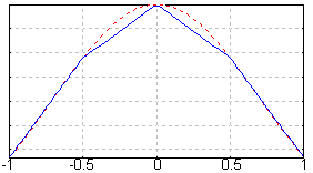
Consider the problem of finding a linear spline for
with the following knots
After directly applying the spline formula, we get the following spline::
The spline function (blue lines) and the function it is approximating (red dashes) are graphed below:

![S(x) = \left\{\begin{matrix}
S_0(x) & x \in [x_0, x_1] \\
S_1(x) & x \in [x_1, x_2] \\
\vdots & \vdots \\
S_{n-1}(x) & x \in [x_{n-1}, x_n]
\end{matrix}\right.](http://upload.wikimedia.org/math/2/5/b/25b21a5e9c133f7e2e1b7c87c53c458f.png)


![S(x)=\left\{\begin{matrix} S_0(x),\ x\in[x_0,x_1]\\ S_1(x),\ x\in[x_1,x_2]\\ \cdots \\ S_{n-1}(x),\ x\in[x_{n-1},x_n]\end{matrix}\right.](http://upload.wikimedia.org/math/2/1/6/2166a209adfb6a6140e6a86c22c2a199.png)


![S(x) = \left\{\begin{matrix}
e^{-1} + 2(e^{-\frac{1}{4}} - e^{-1})(x+1) & x \in [-1, -\frac{1}{2}] \\
e^{-\frac{1}{4}} + 2(1-e^{-\frac{1}{4}})(x+\frac{1}{2}) & x \in [-\frac{1}{2},0] \\
1 + 2(e^{-\frac{1}{4}}-1)x & x \in [0,\frac{1}{2}] \\
e^{-\frac{1}{4}} + 2(e^{-1} - e^{-\frac{1}{4}})(x-\frac{1}{2}) & x \in [\frac{1}{2},1] \\
\end{matrix}\right.](http://upload.wikimedia.org/math/a/9/b/a9b4fec5ecdf76f0b71e9c35c17c8749.png)


