Lagrangian mechanics

	Classical mechanics
	; Newton's Second Law
Fundamental concepts
	Space · Time · Mass · Force; Energy · Momentum;
Formulations
	Newtonian mechanics; Lagrangian mechanics; Hamiltonian mechanics;
Branches
	Statics; Dynamics; Kinematics; Applied mechanics; Celestial mechanics; Continuum mechanics; Statistical mechanics
Scientists
	Newton · Euler · d'Alembert · Clairaut; Lagrange · Laplace · Hamilton · Poisson;
	This box: view • talk • edit

From Wikipedia, the free encyclopedia

Jump to: navigation, search

Lagrangian mechanics is a re-formulation of classical mechanics that combines conservation of momentum with conservation of energy. It was introduced by Italian mathematician Lagrange in 1788. In Lagrangian mechanics, the trajectory of a system of particles is derived by solving Lagrange's equation, given herein, for each of the system's generalized coordinates. The fundamental lemma of the calculus of variations shows that solving Lagrange's equation is equivalent to finding the path that minimizes the action functional, a quantity that is the integral of the Lagrangian over time.

The use of generalized coordinates may considerably simplify a system's analysis. For example, consider a small frictionless bead traveling in a groove. If one is tracking the bead as a particle, calculation of the motion of the bead using Newtonian mechanics would require solving for the time-varying constraint force required to keep the bead in the groove. For the same problem using Lagrangian mechanics, one looks at the path of the groove and chooses a set of independent generalized coordinates that completely characterize the possible motion of the bead. This choice eliminates the need for the constraint force to enter into the resultant system of equations. There are fewer equations since one is not directly calculating the influence of the groove on the bead at a given moment.

[edit] Lagrange's equations

The equations of motion in Lagrangian mechanics are Lagrange's equations, also known as Euler–Lagrange equations. Below, we sketch out the derivation of Lagrange's equation. Please note that in this context, V is used rather than U for potential energy and T replaces K for kinetic energy. See the references for more detailed and more general derivations.

Start with D'Alembert's principle for the virtual work of applied forces, $\mathbf{F}_i$ , and inertial forces on a three dimensional accelerating system of n particles, i, whose motion is consistent with its constraints:^[1]^:269

$\delta W = \sum_{i=1}^n ( \mathbf {F}_{i} - m_i \mathbf{a}_i )\cdot \delta \mathbf r_i = 0$ .

δ W

is the virtual work

$\delta \mathbf r_i$ is the virtual displacement of the system, consistent with the constraints

m i

are the masses of the particles in the system

$\mathbf a_i$ are the accelerations of the particles in the system

$m_i \mathbf a_i$ together as products represent the time derivatives of the system momenta, aka. inertial forces

i

is an integer used to indicate (via subscript) a variable corresponding to a particular particle

n

is the number of particles under consideration

Break out the two terms:

$\delta W = \sum_{i=1}^n \mathbf {F}_{i} \cdot \delta \mathbf r_i - \sum_{i=1}^n m_i \mathbf{a}_i \cdot \delta \mathbf r_i = 0$ .

Assume that the following transformation equations from m independent generalized coordinates, $q j$ , hold:^[1]^:260

$\mathbf{r}_1=\mathbf{r}_1(q_1, q_2, ..., q_m, t)$ ,

$\mathbf{r}_2=\mathbf{r}_2(q_1, q_2, ..., q_m, t)$ , ...

$\mathbf{r}_n=\mathbf{r}_n(q_1, q_2, ..., q_m, t)$ .

m

(without a subscript) indicates the total number generalized coordinates

An expression for the virtual displacement (differential), $\delta \mathbf{r}_i$ of the system for time-independent constraints is^[1]^:264

$\delta \mathbf{r}_i = \sum_{j=1}^m \frac {\partial \mathbf {r}_i} {\partial q_j} \delta q_j$ .

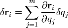j

is an integer used to indicate (via subscript) a variable corresponding to a generalized coordinate

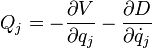
The applied forces may be expressed in the generalized coordinates as generalized forces, $Q j$ ,^[1]^:265

$Q_j = \sum_{i=1}^n \mathbf {F}_{i} \cdot \frac {\partial \mathbf {r}_i} {\partial q_j}$ .

Combining the equations for $δ W$ , $\delta \mathbf{r}_i$ , and $Q j$ yields the following result after pulling the sum out of the dot product in the second term:^[1]^:269

$\delta W = \sum_{j=1}^m Q_j \delta q_j - \sum_{j=1}^m \sum_{i=1}^n m_i \mathbf{a}_i \cdot \frac {\partial \mathbf {r}_i} {\partial q_j} \delta q_j = 0$ .

Substituting in the result from the kinetic energy relations to change the inertial forces into a function of the kinetic energy leaves^[1]^:270

$\delta W = \sum_{j=1}^m Q_j \delta q_j - \sum_{j=1}^m \left ( \frac {d}{d t} \left ( \frac {\partial T}{\partial \dot{q}_j} \right ) - \frac {\partial T}{\partial q_j} \right ) \delta q_j = 0$ .

In the above equation, $δ q j$ is arbitrary, though it is—by definition—consistent with the constraints. So the relation must hold term-wise:^[1]^:270

$Q_j = \frac {d}{d t} \left ( \frac {\partial T}{\partial \dot{q}_j} \right ) - \frac {\partial T}{\partial q_j}$ .

If the $\mathbf F_i$ are conservative, they may be represented by a scalar potential field, $V$ :^[1]^{:266 & 270}

$\mathbf F_i = - \nabla V \Rightarrow Q_j = - \sum_{i=1}^n \nabla V \cdot \frac {\partial \mathbf {r}_i} {\partial q_j} = - \frac {\partial V}{\partial q_j}$ .

The previous result may be easier to see by recognizing that $V$ is a function of the $\mathbf {r}_i$ , which are in turn functions of $q j$ , and then applying the chain rule to the derivative of $V$ with respect to $q j$ .

The definition of the Lagrangian is^[1]^:270

$\mathcal{L} = T - V$ .

Since the potential field is only a function of position, not velocity, Lagrange's equations are as follows:^[1]^:270

$0 = \frac {d}{d t} \left ( \frac {\partial \mathcal L}{\partial \dot{q}_j} \right ) - \frac {\partial \mathcal L}{\partial q_j}$ .

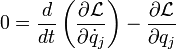This is consistent with the results derived above and may be seen by differentiating the right side of the Lagrangian with respect to $\dot{q}_j$ and time, and solely with respect to $q j$ , adding the results and associating terms with the equations for $\mathbf F_i$ and $Q j$ .

In a more general formulation, the forces could be both potential and viscous. If an appropriate transformation can be found from the $\mathbf F_i$ , Rayleigh suggests using a dissipation function, $D$ , of the following form:^[1]^:271

$D = \frac {1}{2} \sum_{j=1}^m \sum_{k=1}^m C_{j k} \dot{q}_j \dot{q}_k$ .

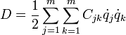C j k

are constants that are related to the damping coefficients in the physical system, though not necessarily equal to them

If $D$ is defined this way, then^[1]^:271

$Q_j = - \frac {\partial V}{\partial q_j} - \frac {\partial D}{\partial \dot{q}_j}$ and

$0 = \frac {d}{d t} \left ( \frac {\partial \mathcal L}{\partial \dot{q}_j} \right ) - \frac {\partial \mathcal L}{\partial q_j} + \frac {\partial D}{\partial \dot{q}_j}$ .

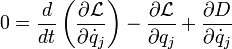[edit] Kinetic energy relations

The kinetic energy, $T$ , for the system of particles is defined by^[1]^:269

$T = \frac {1}{2} \sum_{i=1}^n m_i \mathbf {v}_i \cdot \mathbf {v}_i$ .

The partial derivative of $T$ with respect to the time derivatives of the generalized coordinates, $\dot{q}_j$ , is^[1]^:269

$\frac {\partial T}{\partial \dot{q}_j} = \sum_{i=1}^n m_i \mathbf {v}_i \cdot \frac {\partial \mathbf {v}_i} {\partial \dot{q}_j}$ .

The previous result may be difficult to visualize. As a result of the product rule, the derivative of a general dot product $\frac{d}{dx} ( \mathbf{f}(x) \cdot \mathbf{g}(x) )$ is $\mathbf{f}(x) \cdot \frac{d}{dx} \mathbf{g}(x) + \mathbf{g}(x) \cdot \frac{d}{dx} \mathbf{f}(x)$ This general result may be seen by briefly stepping into a Cartesian coordinate system, recognizing that the dot product is (there) a term-by-term product sum, and also recognizing that the derivative of a sum is the sum of its derivatives. In our case, f and g are equal to v, which is why the factor of one half disappears.

According to the chain rule and the coordinate transformation equations given above for $\mathbf{r}$ , its time derivative, $\mathbf{v}$ , is:^[1]^:264

$\mathbf{v}_i = \sum_{k=1}^m \frac {\partial \mathbf{r}_i}{\partial q_k} \dot{q}_k + \frac {\partial \mathbf{r}_i}{\partial t}$ .

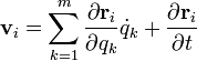Together, the definition of $\mathbf v_i$ and the total differential, $d \mathbf {r}_i$ , suggest that^[1]^:269

$\frac {\partial \mathbf {v}_i}{\partial \dot{q}_j} = \frac {\partial \mathbf {r}_i}{\partial q_j}$ .

[ Remember that : $\frac {\partial } {\partial {\dot{q}_k}} {A}{\dot{q}_k} = A$ . Also remember that in the sum, there is only one ${\dot{q}_j}$ . ]

Substituting this relation back into the expression for the partial derivative of $T$ gives^[1]^:269

$\frac {\partial T}{\partial \dot{q}_j} = \sum_{i=1}^n m_i \mathbf v_i \cdot \frac {\partial \mathbf {r}_i}{\partial q_j}$ .

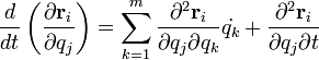
Taking the time derivative gives^[1]^:270

$\frac {d}{d t} \left ( \frac {\partial T}{\partial \dot{q}_j} \right ) = \sum_{i=1}^n \left [ m_i \mathbf a_i \cdot \frac {\partial \mathbf {r}_i}{\partial q_j} + m_i \mathbf {v}_i \cdot \frac {d}{d t} \left ( \frac {\partial \mathbf {r}_i}{\partial q_j} \right ) \right ]$ .

Using the chain rule on the last term gives^[1]^:270

$\frac {d}{d t} \left ( \frac {\partial \mathbf {r}_i}{\partial q_j} \right ) = \sum_{k=1}^m \frac {\partial^2 \mathbf r_i}{\partial q_j \partial q_k} \dot{q_k} + \frac {\partial^2 \mathbf r_i}{\partial q_j \partial t}$ .

From the expression for $\mathbf v_i$ , one sees that^[1]^:270

$\frac {d}{d t} \left ( \frac {\partial \mathbf {r}_i}{\partial q_j} \right ) = \frac {\partial \mathbf {v}_i}{\partial q_j}$ .

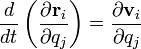This allows simplification of the last term,^[1]^:270

$\frac {d}{d t} \left ( \frac {\partial T}{\partial \dot{q}_j} \right ) = \sum_{i=1}^n \left [ m_i \mathbf a_i \cdot \frac {\partial \mathbf {r}_i}{\partial q_j} + m_i \mathbf {v}_i \cdot \frac {\partial \mathbf {v}_i}{\partial q_j} \right ]$ .

The partial derivative of $T$ with respect to the generalized coordinates, $q j$ , is^[1]^:270

$\frac {\partial T}{\partial q_j} = \sum_{i=1}^{n} \frac { \partial [ \frac{1}{2} m_i {v_i}^{2} ] }{\partial q_j} = \sum_{i=1}^{n} \frac { \partial [ \frac{1}{2} m_i \ ( \mathbf {v}_i \cdot \mathbf {v}_i ) ] }{\partial q_j} = \! \frac{1}{2} \sum_{i=1}^{n} \left[ m_i \mathbf {v}_i \cdot \frac {\partial \mathbf {v}_i}{\partial q_j} + m_i \mathbf {v}_i \cdot \frac {\partial \mathbf {v}_i} {\partial q_j} \right] = \sum_{i=1}^{n}m_i \mathbf {v}_i \cdot \frac {\partial \mathbf {v}_i}{\partial q_j}$ .

[This last result may be obtained by doing a partial differentiation directly on the kinetic energy definition represented by the first equation.] The last two equations may be combined to give an expression for the inertial forces in terms of the kinetic energy:^[1]^:270

$\frac {d}{d t} \left ( \frac {\partial T}{\partial \dot{q}_j} \right ) - \frac {\partial T}{\partial q_j} = \sum_{i=1}^n m_i \mathbf a_i \cdot \frac {\partial \mathbf {r}_i}{\partial q_j}$

[edit] Old Lagrange's equations

Consider a single particle with mass m and position vector $\bold{r}$ , moving under an applied force, $\bold{F}$ , which can be expressed as the gradient of a scalar potential energy function $V (\bold{r},t)$ :

$\bold{F} = - \bold{\nabla} V.$

Such a force is independent of third- or higher-order derivatives of $\bold{r}$ , so Newton's second law forms a set of 3 second-order ordinary differential equations. Therefore, the motion of the particle can be completely described by 6 independent variables, or degrees of freedom. An obvious set of variables is $\{ \bold{r}_j, \dot{\bold{r}}_j | j = 1, 2, 3\}$ , the Cartesian components of $\bold{r}$ and their time derivatives, at a given instant of time (i.e. position (x,y,z) and velocity $(v x, v y, v z)$ ).

More generally, we can work with a set of generalized coordinates, $q j$ , and their time derivatives, the generalized velocities, $\dot{q_j}$ . The position vector, $\bold{r}$ , is related to the generalized coordinates by some transformation equation:

$\bold{r} = \bold{r}(q_i , q_j , q_k, t).$

For example, for a simple pendulum of length l, a logical choice for a generalized coordinate is the angle of the pendulum from vertical, θ, for which the transformation equation would be

$\bold{r}(\theta, \dot{\theta} , t) = (l \sin \theta, l \cos \theta)$ .

The term "generalized coordinates" is really a holdover from the period when Cartesian coordinates were the default coordinate system.

Consider an arbitrary displacement $\delta \bold{r}$ of the particle. The work done by the applied force $\bold{F}$ is $W = \bold{F} \cdot \delta \bold{r}$ . Using Newton's second law, we write:

$\begin{matrix} \bold{F} \cdot \delta \bold{r} = m\ddot{\bold{r}} \cdot \delta \bold{r}. \end{matrix}$

Since work is a physical scalar quantity, we should be able to rewrite this equation in terms of the generalized coordinates and velocities. On the left hand side,

$\begin{matrix} \bold{F} \cdot \bold{\delta} \bold{r} & = & - \bold{\nabla} V \cdot \displaystyle\sum_i {\partial \bold{r} \over \partial q_i} \delta q_i \\ \\ & = & - \displaystyle\sum_{i,j} {\partial V \over \partial r_j} {\partial r_j \over \partial q_i} \delta q_i \\ \\ & = & - \displaystyle\sum_i {\partial V \over \partial q_i} \delta q_i. \\ \end{matrix}$

On the right hand side, carrying out a change of coordinates^{[clarification needed]}, we obtain:

$m \ddot{\bold{r}} \cdot \delta \bold{r} = m \sum_{i,j} \ddot{r_i} {\partial r_i \over \partial q_j} \delta q_j$

Rearranging Slightly:

$m \ddot{\bold{r}} \cdot \delta \bold{r} = m \sum_j \left[ \sum_i \ddot{r_i} {\partial r_i \over \partial q_j} \right] \delta q_j$

Now, by performing an "integration by parts" transformation, with respect to t:

$m \ddot{\bold{r}} \cdot \delta \bold{r} = m \sum_j \left[ \sum_i \left[ {\mathrm{d} \over \mathrm{d}t} \left( \dot{r_i} {\partial r_i \over \partial q_j} \right) - \dot{r_i} {\mathrm{d} \over \mathrm{d}t}\left( {\partial r_i \over \partial q_j} \right) \right] \right] \delta q_j$

Recognizing that ${\mathrm{d} \over \mathrm{d}t}{\partial r_j \over \partial q_i} = {\partial \dot{r_j} \over \partial q_i}$ and ${\partial r_j \over \partial q_i} = {\partial \dot{r_j} \over \partial \dot{q_i}}$ , we obtain:

$m \ddot{\bold{r}} \cdot \delta \bold{r} = m \sum_j \left[ \sum_i \left[ {\mathrm{d} \over \mathrm{d}t} \left( \dot{r_i} {\partial \dot{r_i} \over \partial \dot{q_j}} \right) - \dot{r_i} {\partial \dot{r_i} \over \partial q_j} \right] \right] \delta q_j$

Now, by changing the order of differentiation, we obtain:

$m \ddot{\bold{r}} \cdot \delta \bold{r} = m \sum_j \left[ \sum_i \left[ {\mathrm{d} \over \mathrm{d}t} {\partial \over \partial \dot{q_j}} \left( \frac{1}{2} \dot{r_i}^2 \right) - {\partial \over \partial q_j} \left( \frac{1}{2} \dot{r_i}^2 \right) \right] \right] \delta q_j$

Finally, we change the order of summation:

$m \ddot{\bold{r}} \cdot \delta \bold{r} = \sum_j \left[ {\mathrm{d} \over \mathrm{d}t} {\partial \over \partial \dot{q_j}} \left( \sum_i \frac{1}{2} m \dot{r_i}^2 \right) - {\partial \over \partial q_j} \left( \sum_i \frac{1}{2} m \dot{r_i}^2 \right) \right] \delta q_j$

Which is equivalent to:

$m \ddot{\bold{r}} \cdot \delta \bold{r} = \sum_i \left[{\mathrm{d} \over \mathrm{d}t}{\partial T \over \partial \dot{q_i}}-{\partial T \over \partial q_i}\right]\delta q_i$

where $T=\frac{1}{2}m\dot{\bold{r}}\cdot\dot{\bold{r}}$ is the kinetic energy of the particle. Our equation for the work done becomes

$\sum_i \left[{\mathrm{d} \over \mathrm{d}t}{\partial{T}\over \partial{\dot{q_i}}}-{\partial{(T-V)}\over \partial q_i}\right] \delta q_i = 0.$

However, this must be true for any set of generalized displacements $δ q i$ , so we must have

$\left[ {\mathrm{d} \over \mathrm{d}t}{\partial{T}\over \partial{\dot{q_i}}}-{\partial{(T-V)}\over \partial q_i}\right] = 0$

for each generalized coordinate $δ q i$ . We can further simplify this by noting that V is a function solely of r and t, and r is a function of the generalized coordinates and t. Therefore, V is independent of the generalized velocities:

${\mathrm{d} \over \mathrm{d}t}{\partial{V}\over \partial{\dot{q_i}}} = 0.$

Inserting this into the preceding equation and substituting L = T - V, called the Lagrangian, we obtain Lagrange's equations:

${\partial{\mathcal{L}}\over \partial q_i} = {\mathrm{d} \over \mathrm{d}t}{\partial{\mathcal{L}}\over \partial{\dot{q_i}}}.$

There is one Lagrange equation for each generalized coordinate q_i. When q_i = r_i (i.e. the generalized coordinates are simply the Cartesian coordinates), it is straightforward to check that Lagrange's equations reduce to Newton's second law.

The above derivation can be generalized to a system of N particles. There will be 6N generalized coordinates, related to the position coordinates by 3N transformation equations. In each of the 3N Lagrange equations, T is the total kinetic energy of the system, and V the total potential energy.

In practice, it is often easier to solve a problem using the Euler–Lagrange equations than Newton's laws. This is because not only may more appropriate generalized coordinates q_i be chosen to exploit symmetries in the system, but constraint forces are replaced with simpler relations.

[edit] Examples

In this section two examples are provided in which the above concepts are applied. The first example establishes that in a simple case, the Newtonian approach and the Lagrangian formalism agree. The second case illustrates the power of the above formalism, in a case which is hard to solve with Newton's laws.

[edit] Falling mass

Consider a point mass m falling freely from rest. By gravity a force F = m g is exerted on the mass (assuming g constant during the motion). Filling in the force in Newton's law, we find $\ddot x = g$ from which the solution

$x(t) = \frac{1}{2} g t^2$

follows (choosing the origin at the starting point). This result can also be derived through the Lagrange formalism. Take x to be the coordinate, which is 0 at the starting point. The kinetic energy is $T = \frac{1}{2} m v^2$ and the potential energy is $V = - m g x$ , hence

$\mathcal{L} = T - V = \frac{1}{2} m \dot{x}^2 + m g x$ .

Now we find

$0 = \frac{\partial \mathcal{L}}{\partial x} - \frac{\mathrm{d}}{\mathrm{d}t} \frac{\partial \mathcal{L}}{\partial \dot x} = m g - m \frac{\mathrm{d} \dot x}{\mathrm{d} t}$

which can be rewritten as $\ddot x = g$ , yielding the same result as earlier.

[edit] Pendulum on a movable support

Consider a pendulum of mass m and length l, which is attached to a support with mass M which can move along a line in the x-direction. Let x be the coordinate along the line of the support, and let us denote the position of the pendulum by the angle θ from the vertical. The kinetic energy can then be shown to be

$T = \frac{1}{2} M \dot{x}^2 + \frac{1}{2} m \left( \dot{x}_\mathrm{pend}^2 + \dot{y}_\mathrm{pend}^2 \right) = \frac{1}{2} M \dot{x}^2 + \frac{1}{2} m \left[ \left( \dot x + l \dot\theta \cos \theta \right)^2 + \left( l \dot\theta \sin \theta \right)^2 \right],$

and the potential energy of the system is

$V = m g \operatorname{y}_\mathrm{pend} = - m g l \cos \theta .$

The Lagrangian is therefore

$\mathcal{L} = T - V = \frac{1}{2} M \dot{x}^2 + \frac{1}{2} m \left[ \left( \dot x + l \dot\theta \cos \theta \right)^2 + \left( l \dot\theta \sin \theta \right)^2 \right] + m g l \cos \theta = \frac{1}{2} \left( M + m \right) \dot x^2 + m \dot x l \dot \theta \cos \theta + \frac{1}{2} m l^2 \dot \theta ^2 + m g l \cos \theta$

Sketch of the situation with definition of the coordinates (click to enlarge)

Now carrying out the differentiations gives for the support coordinate x

$\frac{\mathrm{d}}{\mathrm{d}t} \left[ (M + m) \dot x + m l \dot\theta \cos\theta \right] = 0,$

therefore:

$(M + m) \ddot x + m l \ddot\theta\cos\theta-m l \dot\theta ^2 \sin\theta = 0$

indicating the presence of a constant of motion. The other variable yields

$\frac{\mathrm{d}}{\mathrm{d}t}\left[ m( \dot x l \cos\theta + l^2 \dot\theta ) \right] + m (\dot x l \dot \theta + g l) \sin\theta = 0$ ;

therefore

$\ddot\theta + \frac{\ddot x}{l} \cos\theta + \frac{g}{l} \sin\theta = 0$ .

These equations may look quite complicated, but finding them with Newton's laws would have required carefully identifying all forces, which would have been much harder and prone to errors. By considering limit cases ( $\ddot x \to 0$ should give the equations of motion for a pendulum, $\ddot\theta \to 0$ should give the equations for a pendulum in a constantly accelerating system, etc.) the correctness of this system can be verified.

[edit] Hamilton's principle

The action, denoted by $\mathcal{S}$ , is the time integral of the Lagrangian:

$\mathcal{S} = \int \mathcal{L}\,\mathrm{d}t.$

Let q₀ and q₁ be the coordinates at respective initial and final times t₀ and t₁. Using the calculus of variations, it can be shown the Lagrange's equations are equivalent to Hamilton's principle:

The system undergoes the trajectory between t₀ and t₁ whose action has a stationary value.

By stationary, we mean that the action does not vary to first-order for infinitesimal deformations of the trajectory, with the end-points (q₀, t₀) and (q₁,t₁) fixed. Hamilton's principle can be written as:

$\delta \mathcal{S} = 0. \,\!$

Thus, instead of thinking about particles accelerating in response to applied forces, one might think of them picking out the path with a stationary action.

Hamilton's principle is sometimes referred to as the principle of least action. However, this is a misnomer: the action only needs to be stationary, and the correct trajectory could be produced by a maximum, saddle point, or minimum in the action.

We can use this principle instead of Newton's Laws as the fundamental principle of mechanics, this allows us to use an integral principle (Newton's Laws are based on differential equations so they are a differential principle) as the basis for mechanics. However it is not widely stated that Hamilton's principle is a variational principle only with holonomic constraints, if we are dealing with nonholonomic systems then the variational principle should be replaced with one involving d'Alembert principle of virtual work. Working only with holonomic constraints is the price we have to pay for using an elegant variational formulation of mechanics.

[edit] Extensions of Lagrangian mechanics

The Hamiltonian, denoted by H, is obtained by performing a Legendre transformation on the Lagrangian, which introduces new variables, canonically conjugate to the original variables. This doubles the number of variables, but linearizes the differential equations. The Hamiltonian is the basis for an alternative formulation of classical mechanics known as Hamiltonian mechanics. It is a particularly ubiquitous quantity in quantum mechanics (see Hamiltonian (quantum mechanics)).

In 1948, Feynman invented the path integral formulation extending the principle of least action to quantum mechanics for electrons and photons. In this formulation, particles travel every possible path between the initial and final states; the probability of a specific final state is obtained by summing over all possible trajectories leading to it. In the classical regime, the path integral formulation cleanly reproduces Hamilton's principle, and Fermat's principle in optics.

[edit] See also

Canonical coordinates
Functional derivative
Generalized coordinates
Hamiltonian mechanics
Lagrangian analysis (applications of Lagrangian mechanics)
Nielsen form
Restricted three-body problem

[edit] References

^ ^a ^b ^c ^d ^e ^f ^g ^h ⁱ ^j ^k ^l ^m ⁿ ^o ^p ^q ^r ^s ^t ^u ^v ^w Torby, Bruce (1984). "Energy Methods". Advanced Dynamics for Engineers. HRW Series in Mechanical Engineering. United States of America: CBS College Publishing. ISBN 0-03-063366-4.

Goldstein, H. Classical Mechanics, second edition, pp.16 (Addison-Wesley, 1980)
Moon, F. C. Applied Dynamics With Applications to Multibody and Mechatronic Systems, pp. 103-168 (Wiley, 1998).

[edit] Further reading

Landau, L.D. and Lifshitz, E.M. Mechanics, Pergamon Press.
Gupta, Kiran Chandra, Classical mechanics of particles and rigid bodies (Wiley, 1988).

[edit] External links

Tong, David, Classical Dynamics Cambridge lecture notes
Principle of least action interactive Excellent interactive explanation/webpage
Aerospace dynamics lecture notes on Lagrangian mechanics
Aerospace dynamics lecture notes on Rayleigh dissipation function
Introduction to Lagrangian Mechanics [1]
[2] Sydney Grammar School Academic Extension notes

[Torby1984-0] ^ ^a ^b ^c ^d ^e ^f ^g ^h ⁱ ^j ^k ^l ^m ⁿ ^o ^p ^q ^r ^s ^t ^u ^v ^w Torby, Bruce (1984). "Energy Methods". Advanced Dynamics for Engineers. HRW Series in Mechanical Engineering. United States of America: CBS College Publishing. ISBN 0-03-063366-4.

[1]

Lagrangian mechanics

From Wikipedia, the free encyclopedia

Contents

[edit] Lagrange's equations

[edit] Kinetic energy relations

[edit] Old Lagrange's equations

[edit] Examples

[edit] Falling mass

[edit] Pendulum on a movable support

[edit] Hamilton's principle

[edit] Extensions of Lagrangian mechanics

[edit] See also

[edit] References

[edit] Further reading

[edit] External links

Views

Personal tools

Navigation

Search

Interaction

Toolbox

Languages