Gaussian function

From Wikipedia, the free encyclopedia

Normalized Gaussian curves with expected value μ and variance σ². The corresponding parameters are a = 1/(σ√(2π)), b = μ, c = σ

In mathematics, a Gaussian function (named after Carl Friedrich Gauss) is a function of the form:

$f(x) = a e^{- { \frac{(x-b)^2 }{ 2 c^2} } }$

for some real constants a > 0, b, c > 0, and e ≈ 2.718281828 (Euler's number).

The graph of a Gaussian is a characteristic symmetric "bell shape curve" that quickly falls off towards plus/minus infinity. The parameter a is the height of the curve's peak, b is the position of the centre of the peak, and c controls the width of the "bell".

Gaussian functions are widely used in statistics where they describe the normal distributions, in signal processing where they serve to define Gaussian filters, in image processing where two-dimensional Gaussians are used for Gaussian blurs, and in mathematics where they are used to solve heat equations and diffusion equations and to define the Weierstrass transform.

[edit] Properties

Gaussian functions arise by applying the exponential function to a general quadratic function. The Gaussian functions are thus those functions whose logarithm is a quadratic function.

The parameter c is related to the full width at half maximum (FWHM) of the peak according to

$\mathrm{FWHM} = 2 \sqrt{2 \ln 2}\ c = 2.35482\ldots \cdot c.$

Alternatively, the parameter c can be interpreted by saying that the two inflection points of the function occur at x = b − c and x = b + c.

Gaussian functions are analytic, and their limit as $x\to\pm\infty$ is 0.

Gaussian functions are among those functions that are elementary but lack elementary antiderivatives; the integral of the Gaussian function is the error function. Nonetheless their improper integrals over the whole real line can be evaluated exactly, using the Gaussian integral

$\int_{-\infty}^\infty e^{-x^2}\,dx=\sqrt{\pi}$

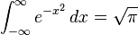
and one obtains

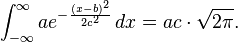
$\int_{-\infty}^\infty a e^{- { (x-b)^2 \over 2 c^2 } }\,dx=ac\cdot\sqrt{2\pi}.$

This integral is 1 if and only if a = 1/(c√(2π)), and in this case the Gaussian is the probability density function of a normally distributed random variable with expected value μ = b and variance σ² = c². These Gaussians are graphed in the accompanying figure.

Taking the Fourier transform of a Gaussian function with parameters a, b = 0 and c yields another Gaussian function, with parameters ac, b = 0 and 1/c. So in particular the Gaussian functions with b = 0 and c = 1 are kept fixed by the Fourier transform (they are eigenfunctions of the Fourier transform with eigenvalue 1).

Gaussian functions centered at zero minimize the Fourier uncertainty principle.

The product of two Gaussian functions is again a Gaussian, and the convolution of two Gaussian functions is again a Gaussian.

[edit] Two-dimensional Gaussian function

Gaussian curve with a 2-dimensional domain

In two-dimensions, one can vary a Gaussian in more parameters: not only may one vary a single width, but one may vary two separate widths, and rotate: one thus obtains both circular Gaussians and elliptical Gaussians, accordingly as the level sets are circles or ellipses.

A particular example of a two-dimensional Gaussian function is

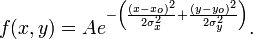
$f(x,y) = A e^{- \left(\frac{(x-x_o)^2}{2\sigma_x^2} + \frac{(y-y_o)^2}{2\sigma_y^2} \right)}.$

Here the coefficient A is the amplitude, x_o,y_o is the center and σ_x, σ_y are the x and y spreads of the blob. The figure on the right was created using A = 1, x_o = 0, y_o = 0, σ_x = σ_y = 1.

In general, a two-dimensional elliptical Gaussian function is expressed as

$f(x,y) = A e^{- \left(a(x - x_o)^2 + 2b(x-x_o)(y-y_o) + c(y-y_o)^2 \right)}$

where the matrix

$\left[\begin{matrix} a & b \\ b & c \end{matrix}\right]$

is positive-definite.

Using this formulation, the figure on the right can be created using A = 1, (x_o, y_o) = (0, 0), a = c = 1, b = 0.

[edit] Meaning of parameters for the general equation

For the general form of the equation the coefficient A is the height of the peak and (x_o, y_o) is the center of the blob.

If we set

$a = \frac{\cos^2\theta}{2\sigma_x^2} + \frac{\sin^2\theta}{2\sigma_y^2}$

$b = -\frac{\sin2\theta}{4\sigma_x^2} + \frac{\sin2\theta}{4\sigma_y^2}$

$c = \frac{\sin^2\theta}{2\sigma_x^2} + \frac{\cos^2\theta}{2\sigma_y^2}$

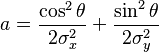
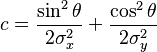
then we rotate the blob by an angle $θ$ . This can be seen in the following examples:

θ = 0

θ = π / 6

θ = π / 3

Using the following MATLAB code one can see the effect of changing the parameters easily

A = 1;
x0 = 0; y0 = 0;
 
sigma_x = 1;
sigma_y = 2;
 
for theta = 0:pi/100:pi
a = cos(theta)^2/2/sigma_x^2 + sin(theta)^2/2/sigma_y^2;
b = -sin(2*theta)/4/sigma_x^2 + sin(2*theta)/4/sigma_y^2 ;
c = sin(theta)^2/2/sigma_x^2 + cos(theta)^2/2/sigma_y^2;
 
[X, Y] = meshgrid(-5:.1:5, -5:.1:5);
Z = A*exp( - (a*(X-x0).^2 + 2*b*(X-x0).*(Y-y0) + c*(Y-y0).^2)) ;
surf(X,Y,Z);shading interp;view(-36,36);axis equal;drawnow
end

Such functions are often used in image processing and in computational models of visual system function -- see the articles on scale space and affine shape adaptation.

Also see multivariate normal distribution.

[edit] Discrete Gaussian

Main article: Discrete Gaussian kernel

The discrete Gaussian kernel (red), compared with the sampled Gaussian kernel (black) for scales

t = .5,1,2,4.

One may ask for a discrete analog to the Gaussian; this is necessary in discrete applications, particularly digital signal processing. A simple answer is to sample the continuous Gaussian, yielding the sampled Gaussian kernel. However, this discrete function does not have the discrete analogs of the properties of the continuous function, and can lead to undesired effects, such as in scale space implementation.

An alternative approach is to use discrete Gaussian kernel:^[1]

$T(n, t) = e^{-t} I_n(t)\,$

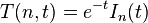
where $I n (t)$ denotes the modified Bessel functions of integer order.

This is the discrete analog of the continuous Gaussian in that it is the solution to the discrete diffusion equation (discrete space, continuous time), just as the continuous Gaussian is the solution to the continuous diffusion equation.

[edit] Applications

Gaussian functions appear in many contexts in the natural sciences, the social sciences, mathematics, and engineering. Some examples include:

In statistics and probability theory, Gaussian functions appear as the density function of the normal distribution, which is a limiting probability distribution of complicated sums, according to the central limit theorem.
Gaussian functions are the Green's function for the (homogeneous and isotropic) diffusion equation (and, which is the same thing, to the heat equation), a partial differential equation that describes the time evolution of a mass-density under diffusion. Specifically, if the mass-density at time t=0 is given by a Dirac delta, which essentially means that the mass is initially concentrated in a single point, then the mass-distribution at time t will be given by a Gaussian function, with the parameter a being linearly related to 1/√t and c being linearly related to √t. More generally, if the initial mass-density is φ(x), then the mass-density at later times is obtained by taking the convolution of φ with a Gaussian function. The convolution of a function with a Gaussian is also known as a Weierstrass transform.
A Gaussian function is the wave function of the ground state of the quantum harmonic oscillator.
The molecular orbitals used in computational chemistry can be linear combinations of Gaussian functions called Gaussian orbitals (see also basis set (chemistry)).
Mathematically, the derivatives of the Gaussian function are the Hermite functions, which are the Gaussian times the Hermite polynomials, up to scale.
Consequently, Gaussian functions are also associated with the vacuum state in quantum field theory.
Gaussian beams are used in optical and microwave systems,
In scale space representation, Gaussian functions are used as smoothing kernels for generating multi-scale representations in computer vision and image processing. Specifically, derivatives of Gaussians (Hermite functions) are used as a basis for defining a large number of types of visual operations.
Gaussian functions are used to define some types of artificial neural networks.
In fluorescence microscopy a 2D Gaussian function is used to approximate the Airy disk, describing the intensity distribution produced by a point source.
In signal processing they serve to define Gaussian filters, such as in image processing where 2D Gaussians are used for Gaussian blurs. In digital signal processing, one uses a discrete Gaussian kernel, which may be defined by sampling a Gaussian, or in a different way.

[edit] See also

[edit] References

^ Lindeberg, T., "Scale-space for discrete signals," PAMI(12), No. 3, March 1990, pp. 234-254.

[edit] External links

Mathworld, includes a proof for the relations between c and FWHM

[tpl90-0] Lindeberg, T., "Scale-space for discrete signals," PAMI(12), No. 3, March 1990, pp. 234-254.

[1]

Gaussian function

From Wikipedia, the free encyclopedia

Contents

[edit] Properties

[edit] Two-dimensional Gaussian function

[edit] Meaning of parameters for the general equation

[edit] Discrete Gaussian

[edit] Applications

[edit] See also

[edit] References

[edit] External links

Views

Personal tools

Navigation

Search

Interaction

Toolbox

Languages