Slide rule
From Wikipedia, the free encyclopedia

The slide rule, also known colloquially as a slipstick[1], is a mechanical analog computer. The slide rule is used primarily for multiplication and division, and also for "scientific" functions such as roots, logarithms and trigonometry, but does not generally perform addition or subtraction.
Slide rules come in a diverse range of styles and generally appear in a linear or circular form with a standardized set of markings (scales) essential to performing mathematical computations. Slide rules manufactured for specialized fields such as aviation or finance typically feature additional scales that aid in calculations common to that field.
William Oughtred and others developed the slide rule in the 1600s based on the emerging work on logarithms by John Napier. Before the advent of the pocket calculator, it was the most commonly used calculation tool in science and engineering. The use of slide rules continued to grow through the 1950s and 1960s even as digital computing devices were being gradually introduced; but around 1974 the electronic scientific calculator made it largely obsolete and most suppliers exited the business.

Contents |
[edit] Basic concepts
In its most basic form, the slide rule uses two logarithmic scales to allow rapid multiplication and division of numbers. These common operations can be time-consuming and error-prone when done on paper. More complex slide rules allow other calculations, such as square roots, exponentials, logarithms, and trigonometric functions.

In general, mathematical calculations are performed by aligning a mark on the sliding central strip with a mark on one of the fixed strips, and then observing the relative positions of other marks on the strips. Numbers aligned with the marks give the approximate value of the product, quotient, or other calculated result.
The user determines the location of the decimal point in the result, based on mental estimation. Scientific notation is used to track the decimal point in more formal calculations. Addition and subtraction steps in a calculation are generally done mentally or on paper, not on the slide rule.
Most slide rules consist of three linear strips of the same length, aligned in parallel and interlocked so that the central strip can be moved lengthwise relative to the other two. The outer two strips are fixed so that their relative positions do not change.
Some slide rules ("duplex" models) have scales on both sides of the rule and slide strip, others on one side of the outer strips and both sides of the slide strip, still others on one side only ("simplex" rules). A sliding cursor with a vertical alignment line is used to find corresponding points on scales that are not adjacent to each other or, in duplex models, are on the other side of the rule. The cursor can also record an intermediate result on any of the scales.
[edit] Operation
[edit] Multiplication
A logarithm transforms the operations of multiplication and division to addition and subtraction according to the rules log(xy) = log(x) + log(y) and log(x / y) = log(x) − log(y). Moving the top scale to the right by a distance of log(x), by matching the beginning of the top scale with the label x on the bottom, aligns each number y, at position log(y) on the top scale, with the number at position log(x) + log(y) on the bottom scale. Because log(x) + log(y) = log(xy), this position on the bottom scale gives xy, the product of x and y. For example, to calculate 3*2, the 1 on the top scale is moved to the 2 on the bottom scale. The answer, 6, is read off the bottom scale where 3 is on the top scale. In general, the 1 on the top is moved to a factor on the bottom, and the answer is read off the bottom where the other factor is on the top.
![]()
Operations may go "off the scale;" for example, the diagram above shows that the slide rule has not positioned the 7 on the upper scale above any number on the lower scale, so it does not give any answer for 2×7. In such cases, the user may slide the upper scale to the left until its right index aligns with the 2, effectively multiplying by 0.2 instead of by 2, as in the illustration below:
![]()
Here the user of the slide rule must remember to adjust the decimal point appropriately to correct the final answer. We wanted to find 2×7, but instead we calculated 0.2×7=1.4. So the true answer is not 1.4 but 14. Resetting the slide is not the only way to handle multiplications that would result in off-scale results, such as 2×7; some other methods are:
- (1) Use the double-decade scales A and B.
- (2) Use the folded scales. In this example, set the left 1 of C opposite the 2 of D. Move the cursor to 7 on CF, and read the result from DF.
- (3) Use the CI inverted scale. Position the 7 on the CI scale above the 2 on the D scale, and then read the result off of the D scale, below the 1 on the CI scale. Since 1 occurs in two places on the CI scale, one of them will always be on-scale.
- (4) Use both the CI inverted scale and the C scale. Line up the 2 of CI with the 1 of D, and read the result from D, below the 7 on the C scale.
Method 1 is easy to understand, but entails a loss of precision. Method 3 has the advantage that it only involves two scales.
[edit] Division
The illustration below demonstrates the computation of 5.5/2. The 2 on the top scale is placed over the 5.5 on the bottom scale. The 1 on the top scale lies above the quotient, 2.75. There is more than one method for doing division, but the method presented here has the advantage that the final result cannot be off-scale, because one has a choice of using the 1 at either end.
![]()
[edit] Other operations
In addition to the logarithmic scales, some slide rules have other mathematical functions encoded on other auxiliary scales. The most popular were trigonometric, usually sine and tangent, common logarithm (log10) (for taking the log of a value on a multiplier scale), natural logarithm (ln) and exponential (ex) scales. Some rules include a Pythagorean scale, to figure sides of triangles, and a scale to figure circles. Others feature scales for calculating hyperbolic functions. On linear rules, the scales and their labeling are highly standardized, with variation usually occurring only in terms of which scales are included and in what order:
| A, B | two-decade logarithmic scales, used for finding square roots and squares of numbers |
| C, D | single-decade logarithmic scales |
| K | three-decade logarithmic scale, used for finding cube roots and cubes of numbers |
| CF, DF | "folded" versions of the C and D scales that start from π rather than from unity; these are convenient in two cases. First when the user guesses a product will be close to 10 but isn't sure whether it will be slightly less or slightly more than 10, the folded scales avoid the possibility of going off the scale. Second, by making the start π rather than the square root of 10, multiplying or dividing by π (as is common in science and engineering formulas) is simplified. |
| CI, DI, DIF | "inverted" scales, running from right to left, used to simplify 1/x steps |
| S | used for finding sines and cosines on the D scale |
| T | used for finding tangents and cotangents on the D and DI scales |
| ST, SRT | used for sines and tangents of small angles and degree–radian conversion |
| L | a linear scale, used along with the C and D scales for finding base-10 logarithms and powers of 10 |
| LLn | a set of log-log scales, used for finding logarithms and exponentials of numbers |
| Ln | a linear scale, used along with the C and D scales for finding natural (base e) logarithms and ex |
|
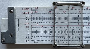
||
| The scales on the front and back of a K&E 4081-3 slide rule. |

The Binary Slide Rule manufactured by Gilson in 1931 performed an addition and subtraction function limited to fractions. [2]
[edit] Roots and powers
There are single-decade (C and D), double-decade (A and B), and triple-decade (K) scales. To compute x2, for example, locate x on the D scale and read its square on the A scale. Inverting this process allows square roots to be found, and similarly for the powers 3, 1/3, 2/3, and 3/2. Care must be taken when the base, x, is found in more than one place on its scale. For instance, there are two nines on the A scale; to find the square root of nine, use the first one; the second one gives the square root of 90.
For xy problems, use the LL scales. When several LL scales are present, use the one with x on it. First, align the leftmost 1 on the C scale with x on the LL scale. Then, find y on the C scale and go down to the LL scale with x on it. That scale will indicate the answer. If y is "off the scale," locate xy / 2 and square it using the A and B scales as described above.
[edit] Trigonometry
The S, T, and ST scales are used for trig functions and multiples of trig functions, for angles in degrees.
For angles from around 5.7 up to 90 degrees, sines are found by comparing the S scale with C. The S scale has a second set of angles (sometimes in a different color), which run in the opposite direction, and are used for cosines. Tangents are found by comparing the T scale with C or, for angles greater than 45 degrees, CI. Common forms such as ksinx can be read directly from x on the S scale to the result on the D scale, when the C-scale index is set at k. For angles below 5.7 degrees, sines, tangents, and radians are approximately equal, and are found on the ST or SRT (sines, radians, and tangents) scale, or simply divided by 57.3 degrees/radian. Inverse trigonometric functions are found by reversing the process.
Many slide rules have S, T, and ST scales marked with degrees and minutes. So-called decitrig models use decimal fractions of degrees instead.
[edit] Logarithms and exponentials
Base-10 logarithms and exponentials are found using the L scale, which is linear. Some slide rules have a Ln scale, which is for base e.
The Ln scale was invented by an 11th grade student, Stephen B. Cohen, in 1958. The original intent was to allow the user to select an exponent x (in the range 0 to 2.3) on the Ln scale and read ex on the C (or D) scale and e–x on the CI (or DI) scale. Pickett, Inc. was given exclusive rights to the scale. Later, the inventor created a set of "marks" on the Ln scale to extend the range beyond the 2.3 limit, but Pickett never incorporated these marks on any of its slide rules.[citation needed]
[edit] Addition and subtraction
Slide rules are not typically used for addition and subtraction, but it is nevertheless possible to do so using two different techniques.[3]
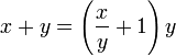
The first method to perform addition and subtraction on the C and D (or any comparable scales) requires converting the problem into one of division. For addition, the quotient of the two variables plus one times the divisor equals their sum:
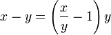
For subtraction, the quotient of the two variables minus one times the divisor equals their difference:
This method is similar to the addition/subtraction technique used for high-speed electronic circuits with the logarithmic number system in specialized computer applications like the Gravity Pipe (GRAPE) supercomputer and hidden Markov models.
The second method utilizes a sliding linear L scale available on some models. Addition and subtraction are performed by sliding the cursor left (for subtraction) or right (for addition) then returning the slide to 0 to read the result.
[edit] Physical design
[edit] Standard linear rules
The length of the slide rule is quoted in terms of the nominal length of the scales. Scales on the most common "10-inch" models are actually 25 cm in length, as they were made to metric standards, though some rules offer slightly extended scales to simplify manipulation when a result overflowed. Pocket rules are typically 5 inches. Models a couple of meters long were sold to be hung in classrooms for teaching purposes. [1]
Typically the divisions mark a scale to a precision of two significant figures, and the user estimates the third figure. Some high-end slide rules have magnifying cursors that make the markings easier to see. Such cursors can effectively double the accuracy of readings, permitting a 10-inch slide rule to serve as well as a 20-inch.
Various other conveniences have been developed. Trigonometric scales are sometimes dual-labeled, in black and red, with complementary angles, the so-called "Darmstadt" style. Duplex slide rules often duplicate some of the scales on the back. Scales are often "split" to get higher accuracy.
Specialized slide rules were invented for various forms of engineering, business and banking. These often had common calculations directly expressed as special scales, for example loan calculations, optimal purchase quantities, or particular engineering equations. For example, the Fisher Controls company distributed a customized slide rule adapted to solving the equations used for selecting the proper size of industrial flow control valves.[citation needed]
[edit] Circular slide rules


Circular slide rules come in two basic types, one with two cursors (left), and another with a movable disk and a single cursor (right). The dual cursor versions perform multiplication and division by maintaining a fixed angle between the cursors as they are rotated around the dial. The single cursor version operates more like the standard slide rule through the appropriate alignment of the scales.
The basic advantage of a circular slide rule is that the longest dimension of the tool was reduced by a factor of about 3 (i.e. by π). For example, a 10 cm circular would have a maximum precision equal to a 30 cm ordinary slide rule. Circular slide rules also eliminate "off-scale" calculations, because the scales were designed to "wrap around"; they never have to be re-oriented when results are near 1.0—the rule is always on scale. However, for non-cyclical non-spiral scales such as S, T, and LL's, the scale length is shortened to make room for end margins.[4]
Circular slide rules are mechanically more rugged and smoother-moving, but their scale alignment precision is sensitive to the centering of a central pivot; a minute 0.1 mm off-centre of the pivot can result in a 0.2 mm worst case alignment error. The pivot, however, does prevent scratching of the face and cursors. The highest accuracy scales are placed on the outer rings. Rather than "split" scales, high-end circular rules use spiral scales for more complex operations like log-of-log scales. One eight-inch premium circular rule had a 50-inch spiral log-log scale.
The main disadvantages of circular slide rules are the difficulty in locating figures along a rotating disc, and limited number of scales. Another drawback of circular slide rules is that less-important scales are closer to the center, and have lower precisions. Most students learned slide rule use on the linear slide rules, and did not find reason to switch.
One slide rule remaining in daily use around the world is the E6B. This is a circular slide rule first created in the 1930s for aircraft pilots to help with dead reckoning. With the aid of scales printed on the frame it also helps with such miscellaneous tasks as converting time, distance, speed, and temperature values, compass errors, and calculating fuel use. The so-called "prayer wheel" is still available in flight shops, and remains widely used. While GPS has reduced the use of dead reckoning for aerial navigation, and handheld calculators have taken over many of its functions, the E6B remains widely used as a primary or backup device and the majority of flight schools demand that their students have some degree of its mastery.
In 1952, Swiss watch company Breitling introduced a pilot's wristwatch with an integrated circular slide rule specialized for flight calculations: the Breitling Navitimer. The Navitimer circular rule, referred to by Breitling as a "navigation computer", featured airspeed, rate/time of climb/descent, flight time, distance, and fuel consumption functions, as well as kilometer–nautical mile and gallon–liter fuel amount conversion functions.
[edit] Cylindrical slide rules

There are two main types of cylindrical slide rules: those with helical scales such as the Fuller, the Otis King and the Bygrave slide rule, and those with bars, such as the Thacher and some Loga models. In either case, the advantage is a much longer scale, and hence potentially higher accuracy, than a straight or circular rule.
[edit] Materials
Traditionally slide rules were made out of hard wood such as mahogany or boxwood with cursors of glass and metal. At least one high precision instrument was made of steel.
In 1895, a Japanese firm, Hemmi, started to make slide rules from bamboo, which had the advantages of being dimensionally stable, strong and naturally self-lubricating. These bamboo slide rules were introduced in Sweden in September, 1933 [2], and probably only a little earlier in Germany. Scales were made of celluloid or plastic. Later slide rules were made of plastic, or aluminum painted with plastic. Later cursors were acrylics or polycarbonates sliding on Teflon bearings.
All premium slide rules had numbers and scales engraved, and then filled with paint or other resin. Painted or imprinted slide rules were viewed as inferior because the markings could wear off. Nevertheless, Pickett, probably America's most successful slide rule company, made all printed scales. Premium slide rules included clever catches so the rule would not fall apart by accident, and bumpers to protect the scales and cursor from rubbing on tabletops. The recommended cleaning method for engraved markings is to scrub lightly with steel-wool. For painted slide rules, and the faint of heart, use diluted commercial window-cleaning fluid and a soft cloth.
[edit] History

The slide rule was invented around 1620–1630, shortly after John Napier's publication of the concept of the logarithm. Edmund Gunter of Oxford developed a calculating device with a single logarithmic scale, which, with additional measuring tools, could be used to multiply and divide. The first description of this scale was published in Paris in 1624 by Edmund Wingate (c.1593 - 1656), an English Mathematician, in a book entitled “L'usage de la reigle de proportion en l'arithmetique & geometrie”. The book contains a double scale on one side of which is a logarithmic scale and on the other a tabular scale. In 1630, William Oughtred of Cambridge invented a circular slide rule, and in 1632 he combined two Gunter rules, held together with the hands, to make a device that is recognizably the modern slide rule. Like his contemporary at Cambridge, Isaac Newton, Oughtred taught his ideas privately to his students, but delayed in publishing them, and like Newton, he became involved in a vitriolic controversy over priority, with his one-time student Richard Delamain and the prior claims of Wingate. Oughtred's ideas were only made public in publications of his student William Forster in 1632 and 1653.
In 1677, Henry Coggeshall created a two-foot folding rule for timber measure, called the Coggeshall slide rule. His design and uses for the tool gave the slide rule purpose outside of mathematical inquiry.
In 1722, Warner introduced the two- and three-decade scales, and in 1755 Everard included an inverted scale; a slide rule containing all of these scales is usually known as a "polyphase" rule.
In 1815, Peter Mark Roget invented the log log slide rule, which included a scale displaying the logarithm of the logarithm. This allowed the user to directly perform calculations involving roots and exponents. This was especially useful for fractional powers.
[edit] Modern form
The more modern form was created in 1859 by French artillery lieutenant Amédée Mannheim, "who was fortunate in having his rule made by a firm of national reputation and in having it adopted by the French Artillery." It was around that time, as engineering became a recognized professional activity, that slide rules came into wide use in Europe. They did not become common in the United States until 1881, when Edwin Thacher introduced a cylindrical rule there. The duplex rule was invented by William Cox in 1891, and was produced by Keuffel and Esser Co. of New York.[5][6]
Astronomical work also required fine computations, and in 19th century Germany a steel slide rule about 2 meters long was used at one observatory. It had a microscope attached, giving it accuracy to six decimal places.
In World War II, bombardiers and navigators who required quick calculations often used specialized slide rules. One office of the U.S. Navy actually designed a generic slide rule "chassis" with an aluminum body and plastic cursor into which celluloid cards (printed on both sides) could be placed for special calculations. The process was invented to calculate range, fuel use and altitude for aircraft, and then adapted to many other purposes.

Throughout the 1950s and 1960s the slide rule was the symbol of the engineer's profession (in the same way that the stethoscope symbolizes the medical profession).[citation needed] German rocket scientist Wernher von Braun brought two 1930s vintage Nestler slide rules with him when he moved to the U.S. after World War II to work on the American space program. Throughout his life he never used any other pocket calculating devices; slide rules served him perfectly well for making quick estimates of rocket design parameters and other figures. Aluminum Pickett-brand slide rules were carried on five Apollo space missions, including to the moon, according to advertising on Pickett's N600 slide rule boxes [3].
Some engineering students and engineers carried ten-inch slide rules in belt holsters, and even into the mid 1970s this was a common sight on campuses. Students also might keep a ten-or twenty-inch rule for precision work at home or the office while carrying a five-inch pocket slide rule around with them.
In 2004, education researchers David B. Sher and Dean C. Nataro conceived a new type of slide rule based on prosthaphaeresis, an algorithm for rapidly computing products that predates logarithms. There has been little practical interest in constructing one beyond the initial prototype, however. [4]
[edit] Decline

The importance of the slide rule began to diminish as electronic computers, a new but very scarce resource in the 1950s, became widely available to technical workers during the 1960s. The introduction of Fortran in 1957 made computers practical for solving modest size mathematical problems. IBM introduced a series of more affordable computers, the IBM 650 (1954), IBM 1620 (1959), IBM 1130 (1965) addressed to the science and engineering market. John Kemeny's BASIC programming language (1964) made it easy for students to use computers. The DEC PDP-8 minicomputer was introduced in 1965.
Computers also changed the nature of calculation. With slide rules, there was a great emphasis on working the algebra to get expressions into the most computable form. Users of slide rules would simply approximate or drop small terms to simplify the calculation. Fortran allowed complicated formulas to be typed in from textbooks without the effort of reformulation. Numerical integration was often easier than trying to find closed form solutions for difficult problems. The young engineer asking for computer time to solve a problem that could have been done by a few swipes on the slide rule became a humorous cliché. Many computer centers had a framed slide rule hung on a wall with the note "In case of emergency, break glass."
Another step toward the replacement of slide rules with electronics was the development of electronic calculators for scientific and engineering use. The first included the Wang Laboratories LOCI-2, [7] introduced in 1965, which used logarithms for multiplication and division and the Hewlett-Packard HP-9100, introduced in 1968. [8] The HP-9100 had trigonometric functions (sin, cos, tan) in addition to exponentials and logarithms. It used the CORDIC (coordinate rotation digital computer) algorithm, [9] which allows for calculation of trigonometric functions using only shift and add operations. This method facilitated the development of ever smaller scientific calculators.
The era of the slide rule ended with the launch of pocket-sized scientific calculators, of which the 1972 Hewlett-Packard HP-35 was the first. Such calculators became known as "slide rule" calculators, since they could perform most, or all the functions of a slide rule. Introduced at US$395, even this was considered expensive for most students. While professional slide rules could also be quite expensive, drug stores often sold basic plastic models for less than $20. But by 1975, basic four-function electronic calculators could be purchased for less than $50. By 1976 the TI-30 offered a scientific calculator for less than $25. After this time, the market for slide rules dwindled quickly as small scientific calculators became affordable.
[edit] Advantages
- A slide rule tends to moderate the fallacy of "false precision" and significance. The typical precision available to a user of a slide rule is about three places of accuracy. This is in good correspondence with most data available for input to engineering formulas. When a modern pocket calculator is used, the precision may be displayed to seven or more decimal places, while in reality the results can never be of greater accuracy than the input data available.
- A slide rule requires a continual estimation of the order of magnitude of the results. On a slide rule 1.5 × 30 (which equals 45) will show the same result as 1,500,000 × 0.03 (which equals 45,000). It is up to the engineer to continually determine the reasonableness of the results, something that can be lost when numbers are carelessly entered into a computer program or a calculator.
- When performing a sequence of multiplications or divisions by the same number, the answer can be often determined by merely glancing at the slide rule without any manipulation. This can be especially useful when calculating percentages, e.g., for test scores, or when comparing prices, e.g., in dollars per kilogram. Multiple speed-time-distance calculations can be performed hands-free at a glance with a slide rule.
- A slide rule does not depend on electricity.
- A slide rule is an easily replicated technology. From a given example of a slide rule, more can be constructed by a competent craftsman from rudimentary materials using non-industrial processes.
- Slide rules are highly standardized, so there is no need to relearn anything when switching to a different rule.
- Slide rules can be made out of cardboard or paper. Many free charts or specialized calculating devices made out of cardboard are actually specialized linear or circular slide rules.
One advantage of using a slide rule together with an electronic calculator is that an important calculation can be checked by doing it on both; because the two instruments are so different, there is little chance of making the same mistake twice.
[edit] Disadvantages
- Errors may arise from mechanical imprecision.
- Calculations using the slide rule are of limited precision due to their analog inputs and outputs. Conversely, because of the discrete numerical input and floating point electronic operations, even modest modern calculators have output resolutions of at least six significant figures.
[edit] Finding and collecting slide rules
There are still people[who?] who prefer a slide rule over an electronic calculator as a practical computing device. Many others keep their old slide rules out of a sense of nostalgia, or collect slide rules as a hobby[5].
A popular model is the Keuffel & Esser Deci-Lon, a premium scientific and engineering slide rule available both in a ten-inch "regular" (Deci-Lon 10) and a five-inch "pocket" (Deci-Lon 5) variant. Another prized American model is the eight-inch Scientific Instruments circular rule. Of European rules, Faber-Castell's high-end models are the most popular among collectors.
Although there is a large supply of slide rules circulating on the market, specimens in good condition tend to be surprisingly expensive. Many rules found for sale on online auction sites are damaged or have missing parts, and the seller may not know enough to supply the relevant information. Replacement parts are scarce, and therefore expensive, and are generally only available for separate purchase on individual collectors' web sites. The Keuffel and Esser rules from the period up to about 1950 are particularly problematic, because the end-pieces on the cursors, made of celluloid, tend to break down chemically over time.
In many cases, an economical method for obtaining a working slide rule is to buy more than one of the same model, and combine their parts.
As of November 2008, the Concise Company in Japan was still commercially manufacturing slide rules (but only circular models).
[edit] See also
| Wikimedia Commons has media related to: Slide rule |
[edit] Notes
- ^ Lester V. Berrey and Melvin van den Bark (1953). American Thesaurus of Slang: A Complete Reference Book of Colloquial Speech. Crowell.
- ^ http://www.sphere.bc.ca/test/circular-man2.html, instruction manual pages 7 & 8. Retrieved March 14, 2007.
- ^ AntiQuark: Slide Rule Tricks
- ^ At least one circular rule, a 1931 Gilson model, sacrificed some of the scales usually found in slide rules in order to obtain additional resolution in multiplication and division. It functioned through the use of a spiral C scale, which was claimed to be 50 feet long and readable to five significant figures. See http://www.sphere.bc.ca/test/gilson/gilson-manual2.jpg. A photo can be seen at http://www.hpmuseum.org/srcirc.htm. An instruction manual for the unit marketed by Dietzgen can be found at http://www.sliderulemuseum.com/SR_Library_General.htm All retrieved March 14, 2007.
- ^ The Log-Log Duplex Decitrig Slide Rule No. 4081: A Manual, Keuffel & Esser, Kells, Kern, and Bland, 1943, p. 92.
- ^ The Polyphase Duplex Slide Rule, A Self-Teaching Manual, Breckenridge, 1922, p.20.
- ^ The Wang LOCI-2
- ^ The HP 9100 Project
- ^ J. E. Volder, "The Birth of CORDIC", J. VLSI Signal Processing 25, 101 (2000).
[edit] External links
General information, history:
- International Slide Rule Museum - Galleries of slide rule scans, downloadable instruction manuals, slide rule encyclopedia and Glossary of Terms, historical dating of specimens, Slide Rule Course, Loaner Slide Rules for Schools, etc.
- History and collection of slide rules Giovanni Pastore - Italy - English version
- The history, theory and use of the engineering slide rule – By Dr James B. Calvert, University of Denver
- Oughtred Society Slide Rule Home Page – Dedicated to the preservation and history of slide rules
- Early Calculators: Slide Rules – At the Museum of HP Calculators
- The Slide Rule Universe – A comprehensive slide rule reference and buying/selling site
- "How a slide rule works" – From the Slide Rule Universe
- "Mad Slide Ruling" – from The Mad Slider Ruler
- International Slide Rule Group – The International Slide Rule Group "ISRG" is devoted to collectors of slide rules and associated mechanical calculating instruments.
- Pastore, Giovanni, Antikythera E I Regoli Calcolatori, Rome, 2006, privately published
- International Slide Rule Museum - Simulator with an Illustrated Self-Guided Course On How To Use The Slide Rule
- Cold War Calculators Slide rules for military and civil defence use.
How-To's:
- International Slide Rule Museum - Illustrated Self-Guided Course On How To Use The Slide Rule (with simulators)
- "Slide rule construction plans" (PDF) – from Scientific American magazine, May 2006 (accompanying an article by Cliff Stoll)
- "Make your own slide rule" (PDF) – By Luis Fernandes, Dept. of Electrical and Computer Engineering, Ryerson University
- "Make your own circular slide rule" – By Dr. Charles Kankelborg, Department of Physics, Montana State University
- How to make your own slide rule, from Sphere Research
- Photo-realistic Aristo Multilog Nr. 970 Slide Rule Simulator, with digital readout of scales to aid learning, by Stefan Vorkoetter
- A Collection of Photo-realistic Pickett Slide Rule Simulators, by Derek Ross
- Lessons and Videos on using the Slide Rule from The Mad Slide Ruler
- A virtual slide rule for kids Includes lessons such as how to add with slide rule, a simple calculus example using mouse and cheese, and more.

