Longest common subsequence problem
From Wikipedia, the free encyclopedia
The longest common subsequence (LCS) problem is to find the longest subsequence common to all sequences in a set of sequences (often just two). It is a classic computer science problem, the basis of diff (a file comparison program that outputs the differences between two files), and has applications in bioinformatics.
Contents |
[edit] Complexity
For the general case of an arbitrary number of input sequences, the problem is NP-hard.[1] When the number of sequences is constant, the problem is solvable in polynomial time by dynamic programming (see Solution below). Assume you have N sequences of lengths  . A naive search would test each of the
  subsequences of the first sequence to determine whether they are also subsequences of the remaining sequences; each subsequence may be tested in time linear in the lengths of the remaining sequences, so the time for this algorithm would be

For the case of two sequences of n and m elements, the running time of the dynamic programming approach is O(n × m). For an arbitrary number of input sequences, the dynamic programming approach gives a solution in

There exist methods with lower complexity,[2] which often depend on the length of the LCS, the size of the alphabet, or both.
Notice that the LCS is not necessarily unique; for example the LCS of "ABC" and "ACB" is both "AB" and "AC". Indeed the LCS problem is often defined to be finding all common subsequences of a maximum length. This problem inherently has higher complexity, as the number of such subsequences is exponential in the worst case,[3] even for only two input strings. It should not be confused with the longest common substring problem (substrings are necessarily contiguous).
[edit] Solution for two sequences
The LCS problem has what is called an "optimal substructure": the problem can be broken down into smaller, simple "subproblems", which can be broken down into yet simpler subproblems, and so on, until, finally, the solution becomes trivial. The LCS problem also has what are called "overlapping subproblems": the solution to a higher subproblem depends on the solutions to several of the lower subproblems. Problems with these two properties—optimal substructure and overlapping substructure—can be approached by a problem-solving technique called dynamic programming, in which the solution is built up starting with the simplest subproblems. The procedure requires what is called "memoization": saving the solutions to one level of subproblem in a table so that the solutions are available to the next level of subproblems. This method is illustrated here.
[edit] Prefixes
The subproblems become simpler as the sequences become shorter. Shorter sequences are conveniently described using the term, prefix. A prefix of a sequence is the sequence with the end cut off. Let S be the sequence (AGCA). Then, a prefix of S is the sequence (AG). Prefixes are denoted with the name of the sequence, followed by a subscript to indicate how many characters the prefix contains.[4] The prefix (AG) is denoted S2, since it contains the first 2 elements of S. The possible prefixes of S are
- S1 = (A)
- S2 = (AG)
- S3 = (AGC)
- S4 = (AGCA)
The solution to the LCS problem for two arbitrary sequences, X and Y, amounts to constructing some function, LCS(X, Y), that gives the longest subsequences common to X and Y. That function relies on the following two properties.
[edit] First property
Suppose that two sequences both end in the same element. To find their LCS, shorten each sequence by removing the last element, find the LCS of the shortened sequences, and to that LCS append the removed element.
- For example, here are two sequences having the same last element: (BANANA) and (ATNA).
- Remove that last element from each: (BANAN) and (ATN)
- The LCS of these last two sequences is, by inspection, (AN).
- Append the removed element, A, giving (ANA), which, by inspection, is the LCS of the original sequences.
In terms of prefixes,
- LCS(Xn, Ym) = (LCS( Xn-1, Ym-1), xn)
where the comma indicates that the following element, xn, is appended to the sequence. Note that the LCS for Xn and Ym involves determining the LCS of the shorter sequences, Xn-1 and Ym-1.
[edit] Second property
Let X and Y be two sequences, where X contains m elements, and Y contains n elements. The final elements of these sequences are not the same. If the last element is removed from each sequence, the shortened sequences are represented by Xm – 1 and Yn – 1.
- The LCS of X and Y are the longest sequences contained in LCS(Xm – 1, Y) and LCS(X, Yn – 1).
| G | A | |
|---|---|---|
| A | Ø | (G) |
| G | (A) |
This is not obvious, so it will be illustrated by considering the LCS of (GA) and (AG). The prefixes of these sequences are placed in the LCS table on the right (only the last element of each prefix is shown). The first cell in the table is for the LCS of (G) and (A); by inspection, this is an empty sequence. The next cell is for the LCS of (G) and (AG); by inspection, the LCS is (G). The third cell is for the LCS of (GA) and (A); by inspection, this is (A). The “second property” can be used to find the LCS for the final cell. Its LCS depends on the solutions to subproblems given in two other cells:
- LCS(X, Y) = the longest sequences of LCS(Xm – 1, Y) and LCS(X, Yn – 1)
Here is the same thing with the Xs and Ys replaced with the sequences applicable to the final cell.
| G | A | |
|---|---|---|
| A | Ø | (G) |
| G | (A) |  (G), (A) (G), (A) |
- LCS((GA), (AG)) = the longest sequences of LCS((G), (AG)) and LCS((GA), (A))
The arrows in the final cell (shown on the right) point to the two cells containing the subproblem solutions, which are (G) and (A).
- LCS((GA), (AG)) = the longest sequences of (G) and (A)
Since both sequences are the same length, both are solutions to the problem.
- LCS((GA), (AG)) = (G) and (A)
By inspection, both (G) and (A) are LCSs of (GA) and (AG), so this second property gives the correct LCS, though somewhat mysteriously.
[edit] LCS function defined
Let two sequences be defined as follows: X = (x1, x2...xm) and Y = (y1, y2...yn). The prefixes of X are X1, 2,...m; the prefixes of Y are Y1, 2,...n. Let LCS(Xi, Yj) represent the set of longest common subsequence of prefixes Xi and Yj. This set of sequences is given by the following.
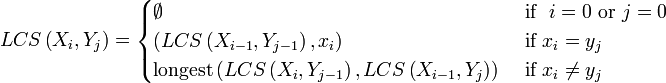
To find the longest subsequences common to Xi and Yj, compare the elements xi and yi. If they are equal, then the sequence LCS(Xi-1, Yj-1) is extended by that element, xi. If they are not equal, then the longest of the two sequences, LCS(Xi, Yj-1), and LCS(Xi-1, Yj), is retained. (If they are both the same length, but not identical, then both are retained.) Notice that the subscripts are reduced by 1 in these formulas. That can result in a subscript of 0. Since the sequence elements are defined to start at 1, it was necessary to add the requirement that the LCS is empty when a subscript is zero.
[edit] Worked example
The longest subsequence common to C = (AGCAT), and R = (GAC) will be found. Because the LCS function uses a "zeroth" element, it is convenient to define zero prefixes that are empty for these sequences: C0 = Ø; and R0 = Ø. All the prefixes are placed in a table with C in the first row (making it a column header) and R in the first column (making it a row header).
| Ø | A | G | C | A | T | |
|---|---|---|---|---|---|---|
| Ø | Ø | Ø | Ø | Ø | Ø | Ø |
| G | Ø | |||||
| A | Ø | |||||
| C | Ø |
This table is used to store the LCS sequence for each step of the calculation. The second column and second row have been filled in with Ø, because when an empty sequence is compared with a non-empty sequence, the longest common subsequence is always an empty sequence.
LCS(R1, C1) is determined by comparing the first elements in each sequence. G and A are not the same, so this LCS gets (using the "second property") the longest of the two sequences, LCS(R1, C0) and LCS(R0, C1). According to the table, both of these are empty, so LCS(R1, C1) is also empty, as shown in the table below. The arrows indicate that the sequence comes from both the cell above, LCS(R0, C1) and the cell on the left, LCS(R1, C0).
LCS(R1, C2) is determined by comparing G and G. They match, so G is appended to the upper left sequence, LCS(R0, C1), which is (Ø), giving (ØG), which is (G).
For LCS(R1, C3), G and C don't match. The sequence above is empty; the one to the left contains one element, G. Selecting the longest of these, LCS(R1, C3) is (G). The arrow points to the left, since that is the longest of the two sequences.
LCS(R1, C4), likewise, is (G).
| Ø | A | G | C | A | T | |
|---|---|---|---|---|---|---|
| Ø | Ø | Ø | Ø | Ø | Ø | Ø |
| G | Ø | Ø |
 (G) (G) |
 (G) (G) |
(G) |
(G) |
| A | Ø | |||||
| C | Ø |
For LCS(R2, C1), A is compared with A. The two elements match, so A is appended to Ø, giving (A).
For LCS(R2, C2), A and G don't match, so the longest of LCS(R1, C2), which is (G), and LCS(R2, C1), which is (A), is used. In this case, they each contain one element, so this LCS is given two subsequences: (A) and (G).
For LCS(R2, C3), A does not match C. LCS(R2, C2) contains sequences (A) and (G); LCS(R1, C3) is (G), which is already contained in LCS(R2, C2). The result is that LCS(R2, C3) also contains the two subsequences, (A) and (G).
For LCS(R2, C4), A matches A, which is appended to the upper left cell, giving (GA).
For LCS(R2, C5), A does not match T. Comparing the two sequences, (GA) and (G), the longest is (GA), so LCS(R2, C5) is (GA).
| Ø | A | G | C | A | T | |
|---|---|---|---|---|---|---|
| Ø | Ø | Ø | Ø | Ø | Ø | Ø |
| G | Ø | Ø |
(G) |
(G) |
(G) |
(G) |
| A | Ø | (A) |
(A) & (G) |
(A) & (G) |
(GA) |
(GA) |
| C | Ø |
For LCS(R3, C1), C and A don't match, so LCS(R3, C1) gets the longest of the two sequences, (A).
For LCS(R3, C2), C and G don't match. Both LCS(R3, C1) and LCS(R2, C2) have one element. The result is that LCS(R3, C2) contains the two subsequences, (A) and (G).
For LCS(R3, C3), C and C match, so C is appended to LCS(R2, C2), which contains the two subsequences, (A) and (G), giving (AC) and (AG).
For LCS(R3, C4), C and A don't match. Combining LCS(R3, C3), which contains (AC) and (GC), and LCS(R2, C4), which contains (GA), gives a total of three sequences: (AC), (GC), and (GA).
Finally, for LCS(R3, C5), C and T don't match. The result is that LCS(R3, C5) also contains the three sequences, (AC), (GC), and (GA).
| Ø | A | G | C | A | T | |
|---|---|---|---|---|---|---|
| Ø | Ø | Ø | Ø | Ø | Ø | Ø |
| G | Ø | Ø |
(G) |
(G) |
(G) |
(G) |
| A | Ø | (A) |
(A) & (G) |
(A) & (G) |
(GA) |
(GA) |
| C | Ø |  (A) (A) |
(A) & (G) |
(AC) & (GC) |
(AC) & (GC) & (GA) |
(AC) & (GC) & (GA) |
The final result is that the last cell contains all the longest subsequences common to (AGCAT) and (GAC); these are (AC), (GC), and (GA). The table also shows the longest common subsequences for every possible pair of prefixes. For example, for (AGC) and (GA), the longest common subsequence are (A) and (G).
[edit] Traceback approach
The calculation the LCS of a row of the LCS table requires only the solutions to the current row and the previous row. Still, for long sequences, these sequences can get numerous and long, requiring a lot of storage space. Storage space can be saved by saving not the actual subsequences, but the length of the subsequence and the direction of the arrows, as in the table below.
| Ø | A | G | C | A | T | |
|---|---|---|---|---|---|---|
| Ø | 0 | 0 | 0 | 0 | 0 | 0 |
| G | 0 | 0 |
1 |
1 |
1 |
1 |
| A | 0 | 1 |
1 |
1 |
2 |
2 |
| C | 0 | 1 |
1 |
2 |
2 |
2 |
The actual subsequences are deduced in a "traceback" procedure that follows the arrows backwards, starting from the last cell in the table. When the length decreases, the sequences must have had a common element. Several paths are possible when two arrows are shown in a cell. Below is the table for such an analysis, with numbers colored in cells where the length is about to decrease. The bold numbers trace out the sequence, (GA).[5]
| Ø | A | G | C | A | T | |
|---|---|---|---|---|---|---|
| Ø | 0 | 0 | 0 | 0 | 0 | 0 |
| G | 0 | 0 |
1 |
1 |
1 |
1 |
| A | 0 | 1 |
1 |
1 |
2 |
2 |
| C | 0 | 1 |
1 |
2 |
2 |
2 |
[edit] Relation to other problems
For two strings  and
and  , the length of the shortest common supersequence is related to the length of the LCS by[2]

The edit distance when only insertion and deletion is allowed (no substitution), or when the cost of the substitution is the double of the cost of an insertion or deletion, is:

[edit] Code for the dynamic programming solution
| The Wikibook Algorithm implementation has a page on the topic of |
[edit] Computing the length of the LCS
The function below takes as input sequences X[1..m] and Y[1..n] computes the LCS between X[1..i] and Y[1..j] for all 1 ≤ i ≤ m and 1 ≤ j ≤ n, and stores it in C[i,j]. C[m,n] will contain the length of the LCS of X and Y.
function  LCSLength(X[1..m], Y[1..n])
    C = array(0..m, 0..n)
    for i := 0..m
       C[i,0] = 0
    for j := 0..n
       C[0,j] = 0
    for i := 1..m
        for j := 1..n
            if X[i] = Y[j]
                C[i,j] := C[i-1,j-1] + 1
            else:
                C[i,j] := max(C[i,j-1], C[i-1,j])
    return C[m,n]
Alternatively, memoization could be used.
[edit] Reading out an LCS
The following function backtraces the choices taken when computing the C table. If the last characters in the prefixes are equal, they must be in an LCS. If not, check what gave the largest LCS of keeping xi and yj, and make the same choice. Just choose one if they were equally long. Call the function with i=m and j=n.
function backTrace(C[0..m,0..n], X[1..m], Y[1..n], i, j)
    if i = 0 or j = 0
        return ""
    else if  X[i-1] = Y[j-1]
        return backTrace(C, X, Y, i-1, j-1) + X[i-1]
    else
        if C[i,j-1] > C[i-1,j]
            return backTrace(C, X, Y, i, j-1)
        else
            return backTrace(C, X, Y, i-1, j)
[edit] Reading out all LCSs
If choosing xi and yj would give an equally long result, read out both resulting subsequences. This is returned as a set by this function. Notice that this function is not polynomial, as it might branch in almost every step if the strings are similar.
function backTraceAll(C[0..m,0..n], X[1..m], Y[1..n], i, j)
    if i = 0 or j = 0
        return {}
    else if X[i] = Y[j]
        return {Z + X[i] for all Z in backTraceAll(C, X, Y, i-1, j-1)}
    else
        R := {}
        if C[i,j-1] ≥ C[i-1,j]
            R := backTraceAll(C, X, Y, i, j-1)
        if C[i-1,j] ≥ C[i,j-1]
            R := R ∪ backTraceAll(C, X, Y, i-1, j)
        return R
[edit] Print the diff
This function will backtrack through the C matrix, and print the diff between the two sequences. Notice that you will get a different answer if you exchange ≥ and <, with > and ≤ below.
function printDiff(C[0..m,0..n], X[1..m], Y[1..n], i, j)
    if i > 0 and j > 0 and X[i] = Y[j]
        printDiff(C, X, Y, i-1, j-1)
        print "  " + X[i]
    else
        if j > 0 and (i = 0 or C[i,j-1] ≥ C[i-1,j])
            printDiff(C, X, Y, i, j-1)
            print "+ " + Y[j]
        else if i > 0 and (j = 0 or C[i,j-1] < C[i-1,j])
            printDiff(C, X, Y, i-1, j)
            print "- " + X[i]
[edit] Example
Let X be "XMJYAUZ" and Y be "MZJAWXU". The longest common subsequence between X and Y is "MJAU". The table C shown below, which is generated by the function LCSlength, shows the lengths of the longest common subsequences between prefixes of X and Y. The ith row and jth column shows the length of the LCS between X1..i and Y1..j.
     | 0 1 2 3 4 5 6 7
     |   M Z J A W X U
-----|-----------------
0    | 0 0 0 0 0 0 0 0
1  X | 0 0 0 0 0 0 1 1
2  M | 0 1 1 1 1 1 1 1
3  J | 0 1 1 2 2 2 2 2
4  Y | 0 1 1 2 2 2 2 2
5  A | 0 1 1 2 3 3 3 3
6  U | 0 1 1 2 3 3 3 4
7  Z | 0 1 2 2 3 3 3 4
The underlined numbers show the path the function backTrack would follow from the bottom right to the top left corner, when reading out an LCS. If the current symbols in X and Y are equal, they are part of the LCS, and we go both up and left. If not, we go up or left, depending on which cell has a higher number. This corresponds to either taking the LCS between X1..i − 1 and Y1..j, or X1..i and Y1..j − 1
[edit] Code optimization
Several optimizations can be made to the algorithm above to speed it up for real-world cases.
[edit] Reduce the problem set
The C matrix in the naive algorithm grows quadratically with the lengths of the sequences. For two 100-item sequences, a 10,000-item matrix would be needed, and 10,000 comparisons would need to be done. In most real-world cases, especially source code diffs and patches, the beginnings and ends of files rarely change, and almost certainly not both at the same time. If only a few items have changed in the middle of the sequence, the beginning and end can be eliminated. This reduces not only the memory requirements for the matrix, but also the number of comparisons that must be done.
function  LCS(X[1..m], Y[1..n])
    m_start := 1
    m_end := m
    n_start := 1
    n_end := n
    trim off the matching items at the beginning
    while m_start ≤ m_end and n_start ≤ n_end and X[m_start] = Y[n_start]
        m_start := m_start + 1
        n_start := n_start + 1
    trim off the matching items at the end
    while m_start ≤ m_end and n_start ≤ n_end and X[m_end] = Y[n_end]
        m_end := m_end - 1
        n_end := n_end - 1
    C = array(m_start-1..m_end, n_start-1..n_end)
    only loop over the items that have changed
    for i := m_start..m_end
        for j := n_start..n_end
            the algorithm continues as before ...
In the best case scenario, a sequence with no changes, this optimization would completely eliminate the need for the C matrix. In the worst case scenario, a change to the very first and last items in the sequence, only two additional comparisons are performed.
[edit] Reduce the comparison time
Most of the time taken by the naive algorithm is spent performing comparisons between items in the sequences. For textual sequences such as source code, you want to view lines as the sequence elements instead of single characters. This can mean comparisons of relatively long strings for each step in the algorithm. Two optimizations can be made that can help to reduce the time these comparisons consume.
[edit] Reduce strings to hashes
A hash function or checksum can be used to reduce the size of the strings in the sequences. That is, for source code where the average line is 60 or more characters long, the hash or checksum for that line might be only 8 to 40 characters long. Additionally, the randomized nature of hashes and checksums would guarantee that comparisons would short-circuit faster, as lines of source code will rarely be changed at the beginning.
There are three primary drawbacks to this optimization. First, an amount of time needs to be spent beforehand to precompute the hashes for the two sequences. Second, additional memory needs to be allocated for the new hashed sequences. However, in comparison to the naive algorithm used here, both of these drawbacks are relatively minimal.
The third drawback is that of collisions. Since the checksum or hash is not guaranteed to be unique, there is a small chance that two different items could be reduced to the same hash. This is unlikely in source code, but it is possible. A cryptographic hash would therefore be far better suited for this optimization, as its entropy is going to be significantly greater than that of a simple checksum. However, the setup and computational requirements of a cryptographic hash may not be worth it for small sequence lengths.
[edit] Reduce strings to identity integers
In source code, there will often be lines that are exactly the same. This could include an empty line between two functions, or a trailing brace, or closing comment, and so on. The algorithm does not need to distinguish between specific instances of these similar lines. That is, one blank line is the same as any other blank line. Therefore, the previous optimization can be taken one step further by reducing each line to an identity integer. String buckets, such as Python dict dictionary objects, Perl hashes, or C++ STL map objects, are well-suited for this optimization.
- Create an empty bucket.
- For each item in the sequence, look to see if it is already present in the bucket.
- If not, add the item to the bucket and tag it with a new identity integer.
- If so, get the identity integer from the bucket.
- Replace the item with its identity integer.
- Repeat.
This method has advantages over the previous optimization. First, it does not suffer from the hash collision problem, as language-specific bucket objects are almost always coded to handle the case of two different items with the same hash. More importantly, each item is reduced from a string to a unique integer, meaning that each comparison is now an integer comparison. There is overhead to the identity allocation, but in terms of the original naive algorithm, this optimization is almost always worth it.
[edit] Reduce the required space
If only the length of the LCS is required, the matrix can be reduced to a 2×min(n,m) matrix with ease, or to min(m,n)+1 vector (smarter) as the dynamic programming approach only needs the current and previous columns of the matrix. Hirschberg's algorithm allows the construction of the optimal sequence itself in the same quadratic time and linear space bounds.[6]
[edit] References
- ^ David Maier (1978). "The Complexity of Some Problems on Subsequences and Supersequences". J. ACM (ACM Press) 25 (2): 322–336. doi:.
- ^ a b L. Bergroth and H. Hakonen and T. Raita (2000). "A Survey of Longest Common Subsequence Algorithms". SPIRE (IEEE Computer Society) 00: 39–48. doi:. ISBN ISBN 0-7695-0746-8.
- ^ Ronald I. Greenberg (2003-08-06). Bounds on the Number of Longest Common Subsequences. v2. http://arxiv.org/abs/cs.DM/0301030.
- ^ Xia, Xuhua (2007). Bioinformatics and the Cell: Modern Computational Approaches in Genomics, Proteomics and Transcriptomics. New York: Springer. p. 24.
- ^ Thomas H. Cormen, Charles E. Leiserson, Ronald L. Rivest and Clifford Stein (2001). "15.4". Introduction to Algorithms (second ed.). MIT Press and McGraw-Hill. pp. 350–355. ISBN 0-262-53196-8.
- ^ Hirschberg, D. S. (1975). "A linear space algorithm for computing maximal common subsequences". Communications of the ACM 18 (6): 341–343. doi:.

