Conjugate gradient method
From Wikipedia, the free encyclopedia

In mathematics, the conjugate gradient method is an algorithm for the numerical solution of particular systems of linear equations, namely those whose matrix is symmetric and positive-definite. The conjugate gradient method is an iterative method, so it can be applied to sparse systems which are too large to be handled by direct methods such as the Cholesky decomposition. Such systems arise regularly when numerically solving partial differential equations.
The conjugate gradient method can also be used to solve unconstrained optimization problems such as energy minimization.
The biconjugate gradient method provides a generalization to non-symmetric matrices. Various nonlinear conjugate gradient methods seek minima of nonlinear equations.
Contents |
[edit] Description of the method
Suppose we want to solve the following system of linear equations
- Ax = b
where the n-by-n matrix A is symmetric (i.e., AT = A), positive definite (i.e., xTAx > 0 for all non-zero vectors x in Rn), and real.
We denote the unique solution of this system by x*.
[edit] The conjugate gradient method as a direct method
We say that two non-zero vectors u and v are conjugate (with respect to A) if

Since A is symmetric and positive definite, the left-hand side defines an inner product

So, two vectors are conjugate if they are orthogonal with respect to this inner product. Being conjugate is a symmetric relation: if u is conjugate to v, then v is conjugate to u. (Note: This notion of conjugate is not related to the notion of complex conjugate.)
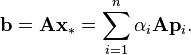
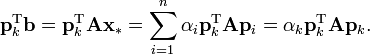
Suppose that {pk} is a sequence of n mutually conjugate directions. Then the pk form a basis of Rn, so we can expand the solution x* of Ax = b in this basis:

The coefficients are given by
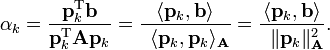
This result is perhaps most transparent by considering the inner product defined above.
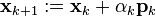
This gives the following method for solving the equation Ax = b. We first find a sequence of n conjugate directions and then we compute the coefficients αk.
[edit] The conjugate gradient method as an iterative method
If we choose the conjugate vectors pk carefully, then we may not need all of them to obtain a good approximation to the solution x*. So, we want to regard the conjugate gradient method as an iterative method. This also allows us to solve systems where n is so large that the direct method would take too much time.
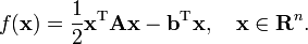
We denote the initial guess for x* by x0. We can assume without loss of generality that x0 = 0 (otherwise, consider the system Az = b − Ax0 instead). Starting with x0 we search for the solution and in each iteration we need a metric to tell us whether we have gotten closer to the solution x* (that is unknown to us). This metric comes from the fact that the solution x* is also the unique minimizer of the following quadratic form; so if f(x) becomes smaller in an iteration it means that we are closer to x*.
This suggests taking the first basis vector p1 to be the gradient of f at x = x0, which equals Ax0−b. Since x0 = 0, this means we take p1 = −b. The other vectors in the basis will be conjugate to the gradient, hence the name conjugate gradient method.
Let rk be the residual at the kth step:

Note that rk is the negative gradient of f at x = xk, so the gradient descent method would be to move in the direction rk. Here, we insist that the directions pk are conjugate to each other, so we take the direction closest to the gradient rk under the conjugacy constraint. This gives the following expression:

(see the picture at the top of the article for the effect of the conjugacy constraint on convergence).
[edit] The resulting algorithm
After some simplifications, this results in the following algorithm for solving Ax = b where A is a real, symmetric, positive-definite matrix. The input vector x0 can be an approximate initial solution or 0.


- repeat


- if rk+1 is sufficiently small then exit loop end if


- end repeat
- The result is xk+1
[edit] Example code of conjugate gradient method in Octave
function [x] = conjgrad(A,b,x0)

   r = b - A*x0;
   w = -r;
   z = A*w;
   a = (r'*w)/(w'*z);
   x = x0 + a*w;
   B = 0;

   for i = 1:size(A)(1);
      r = r - a*z;
      if( norm(r) < 1e-10 )
           break;
      endif
      B = (r'*z)/(w'*z);
      w = -r + B*w;
      z = A*w;
      a = (r'*w)/(w'*z);
      x = x + a*w;
   end

end
[edit] The preconditioned conjugate gradient method
In some cases, preconditioning is necessary to ensure fast convergence of the conjugate gradient method. The preconditioned conjugate gradient method takes the following form:


- repeat


- if rk+1 is sufficiently small then exit loop end if


- end repeat
- The result is xk+1
In the above formulation, M is the preconditioner and has to be symmetric positive-definite. This formulation is equivalent to applying the conjugate gradient method without preconditioning to the system[1]
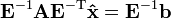
where


[edit] Conjugate gradient on the normal equations
The conjugate gradient method can be applied to an arbitrary n-by-m matrix by applying it to normal equations ATA and right-hand side vector ATb, since ATA is a symmetric positive-semidefinite matrix for any A. The result is conjugate gradient on the normal equations (CGNR).
- ATAx = ATb
As an iterative method, it is not necessary to form ATA explicitly in memory but only to perform the matrix-vector and transpose matrix-vector multiplications. Therefore CGNR is particularly useful when A is a sparse matrix since these operations are usually extremely efficient. However the downside of forming the normal equations is that the condition number κ(ATA) is equal to κ2(A) and so the rate of convergence of CGNR may be slow and the quality of the approximate solution may be sensitive to roundoff errors. Finding a good preconditioner is often an important part of using the CGNR method.
Several algorithms have been proposed (e.g., CGLS, LSQR). The LSQR algorithm purportedly has the best numerical stability when A is ill-conditioned, i.e., A has a large condition number.
[edit] See also
- Biconjugate gradient method (BICG)
- Preconditioned conjugate gradient method (PCG)
- Nonlinear conjugate gradient method
[edit] References
The conjugate gradient method was originally proposed in
- Hestenes, Magnus R.; Stiefel, Eduard (December 1952). "Methods of Conjugate Gradients for Solving Linear Systems" (PDF). Journal of Research of the National Bureau of Standards 49 (6). http://nvl.nist.gov/pub/nistpubs/jres/049/6/V49.N06.A08.pdf.
Descriptions of the method can be found in the following text books:
- Kendell A. Atkinson (1988), An introduction to numerical analysis (2nd ed.), Section 8.9, John Wiley and Sons. ISBN 0-471-50023-2.
- Mordecai Avriel (2003). Nonlinear Programming: Analysis and Methods. Dover Publishing. ISBN 0-486-43227-0.
- Gene H. Golub and Charles F. Van Loan, Matrix computations (3rd ed.), Chapter 10, Johns Hopkins University Press. ISBN 0-8018-5414-8.
[edit] External links
- ^ An Introduction to the Conjugate Gradient Method Without the Agonizing Pain by Jonathan Richard Shewchuk.
- Conjugate Gradient Method by Nadir Soualem.
- Preconditioned conjugate gradient method by Nadir Soualem.
- Iterative methods for sparse linear systems by Yousef Saad
- LSQR: Sparse Equations and Least Squares by Christopher Paige and Michael Saunders.

