Cholesky decomposition

From Wikipedia, the free encyclopedia

In linear algebra, a subfield of mathematics, the Cholesky decomposition is a decomposition of a symmetric, positive-definite matrix into a lower triangular matrix and the transpose of the lower triangular matrix. It was discovered by André-Louis Cholesky. The lower triangular matrix is the Cholesky triangle of the original, positive-definite matrix. Cholesky's result has since been extended to matrices with complex entries. When it is applicable, the Cholesky decomposition is roughly twice as efficient as the LU decomposition for solving systems of linear equations.^[1]

[edit] Statement

If A has real entries and is symmetric (or more generally, is Hermitian) and positive definite, then A can be decomposed as

$\mathbf{A} = \mathbf{L} \mathbf{L}^{*},$

where L is a lower triangular matrix with strictly positive diagonal entries, and L^* denotes the conjugate transpose of L. This is the Cholesky decomposition.

The Cholesky decomposition is unique: given a Hermitian, positive-definite matrix A, there is only one lower triangular matrix L with strictly positive diagonal entries such that A = LL^*. The converse holds trivially: if A can be written as LL^* for some invertible L, lower triangular or otherwise, then A is Hermitian and positive definite.

The requirement that L have strictly positive diagonal entries can be dropped to extend the factorization to the positive semidefinite case. The statement then reads: a square matrix A has a Cholesky decomposition if and only if A is Hermitian and positive semi-definite. Cholesky factorizations for positive semidefinite matrices are not unique in general.

In the special case that A is a symmetric positive-definite matrix with real entries, L can be assumed to have real entries as well.

[edit] Applications

The Cholesky decomposition is mainly used for the numerical solution of linear equations Ax = b. If A is symmetric and positive definite, then we can solve Ax = b by first computing the Cholesky decomposition A = LL^T, then solving Ly = b for y, and finally solving L^Tx = y for x.

[edit] Linear least squares

Systems of the form Ax = b with A symmetric and positive definite arise quite often in applications. For instance, the normal equations in linear least squares problems are of this form. It may also happen that matrix A comes from an energy functional which must be positive from physical considerations; this happens frequently in the numerical solution of partial differential equations.

[edit] Monte Carlo simulation

The Cholesky decomposition is commonly used in the Monte Carlo method for simulating systems with multiple correlated variables: The matrix of inter-variable correlations is decomposed, to give the lower-triangular L. Applying this to a vector of uncorrelated simulated shocks, u, produces a shock vector Lu with the covariance properties of the system being modeled.

[edit] Kalman filters

Unscented Kalman filters commonly use the Cholesky decomposition to choose a set of so-called sigma points. The Kalman filter tracks the average state of a system as a vector x of length N and covariance as an N-by-N matrix P. The matrix P is always positive semi-definite, and can be decomposed into LL^T. The columns of L can be added and subtracted from the mean x to form a set of 2N vectors called sigma points. These sigma points completely capture the mean and covariance of the system state.

[edit] Computing the Cholesky decomposition

There are various methods for calculating the Cholesky decomposition. The algorithms described below all involve about n³/3 FLOPs, where n is the size of the matrix A. Hence, they are half the cost of the LU decomposition, which uses 2n³/3 FLOPs (see Trefethen and Bau 1997).

Which of the algorithms below is faster depends on the details of the implementation. Generally, the first algorithm will be slightly slower because it accesses the data in a more irregular manner.

[edit] The Cholesky algorithm

The Cholesky algorithm, used to calculate the decomposition matrix L, is a modified version of Gaussian elimination.

The recursive algorithm starts with i := 1 and

$\mathbf{A}^{(1)} := \mathbf{A}.$

At step i, the matrix A⁽ⁱ⁾ has the following form:

$\mathbf{A}^{(i)} = \begin{pmatrix} \mathbf{I}_{i-1} & 0 & 0 \\ 0 & a_{i,i} & \mathbf{b}_{i}^{*} \\ 0 & \mathbf{b}_{i} & \mathbf{B}^{(i)} \end{pmatrix},$

where I_i−1 denotes the identity matrix of dimension i − 1.

If we now define the matrix L_i by

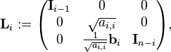
$\mathbf{L}_{i} := \begin{pmatrix} \mathbf{I}_{i-1} & 0 & 0 \\ 0 & \sqrt{a_{i,i}} & 0 \\ 0 & \frac{1}{\sqrt{a_{i,i}}} \mathbf{b}_{i} & \mathbf{I}_{n-i} \end{pmatrix},$

then we can write A⁽ⁱ⁾ as

$\mathbf{A}^{(i)} = \mathbf{L}_{i} \mathbf{A}^{(i+1)} \mathbf{L}_{i}^{*}$

where

$\mathbf{A}^{(i+1)} = \begin{pmatrix} \mathbf{I}_{i-1} & 0 & 0 \\ 0 & 1 & 0 \\ 0 & 0 & \mathbf{B}^{(i)} - \frac{1}{a_{i,i}} \mathbf{b}_{i} \mathbf{b}_{i}^{*} \end{pmatrix}.$

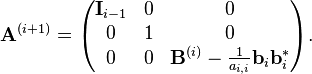
Note that b_i b_i^* is an outer product, therefore this algorithm is called the outer product version in (Golub & Van Loan).

We repeat this for i from 1 to n. After n steps, we get A⁽ⁿ⁺¹⁾ = I. Hence, the lower triangular matrix L we are looking for is calculated as

$\mathbf{L} := \mathbf{L}_{1} \mathbf{L}_{2} \dots \mathbf{L}_{n}.$

[edit] The Cholesky-Banachiewicz and Cholesky-Crout algorithms

If we write out the equation A = LL^*,

${\mathbf{A=LL^T}} = \begin{pmatrix} L_{11} & 0 & 0 \\ L_{21} & L_{22} & 0 \\ L_{31} & L_{32} & L_{33}\\ \end{pmatrix} \begin{pmatrix} L_{11} & L_{21} & L_{31} \\ 0 & L_{22} & L_{32} \\ 0 & 0 & L_{33}\\ \end{pmatrix} = \begin{pmatrix} L_{11}^2 & &(symmetrical) \\ L_{21}L_{11} & L_{21}^2 + L_{22}^2& \\ L_{31}L_{11} & L_{31}L_{21}+L_{32}L_{22} & L_{31}^2 + L_{32}^2+L_{33}^2 \\ \end{pmatrix}$

we obtain the following formula for the entries of L:

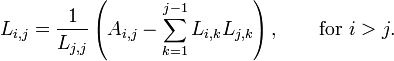
$L_{i,j} = \frac{1}{L_{j,j}} \left( A_{i,j} - \sum_{k=1}^{j-1} L_{i,k} L_{j,k} \right), \qquad\mbox{for } i>j.$

$L_{i,i} = \sqrt{ A_{i,i} - \sum_{k=1}^{i-1} L_{i,k}^2 }.$

The expression under the square root is always positive if A is real and positive-definite.

For complex Hermitian matrix, the following formula applies:

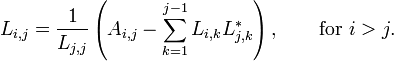
$L_{i,j} = \frac{1}{L_{j,j}} \left( A_{i,j} - \sum_{k=1}^{j-1} L_{i,k} L_{j,k}^* \right), \qquad\mbox{for } i>j.$

$L_{i,i} = \sqrt{ A_{i,i} - \sum_{k=1}^{i-1} L_{i,k}L_{i,k}^* }.$

So we can compute the (i, j) entry if we know the entries to the left and above. The computation is usually arranged in either of the following orders.

The Cholesky-Banachiewicz algorithm starts from the upper left corner of the matrix L and proceeds to calculate the matrix row by row.
The Cholesky-Crout algorithm starts from the upper left corner of the matrix L and proceeds to calculate the matrix column by column.

[edit] Stability of the computation

Suppose that we want to solve a well-conditioned system of linear equations. If the LU decomposition is used, then the algorithm is unstable unless we use some sort of pivoting strategy. In the latter case, the error depends on the so-called growth factor of the matrix, which is usually (but not always) small.

Now, suppose that the Cholesky decomposition is applicable. As mentioned above, the algorithm will be twice as fast. Furthermore, no pivoting is necessary and the error will always be small. Specifically, if we want to solve Ax = b, and y denotes the computed solution, then y solves the disturbed system (A + E)y = b where

$\|\mathbf{E}\|_2 \le c_n \varepsilon \|\mathbf{A}\|_2.$

Here, || ||₂ is the matrix 2-norm, c_n is a small constant depending on n, and ε denotes the unit round-off.

There is one small problem with the Cholesky decomposition. Note that we must compute square roots in order to find the Cholesky decomposition. If the matrix is real symmetric and positive definite, then the numbers under the square roots are always positive in exact arithmetic. Unfortunately, the numbers can become negative because of round-off errors, in which case the algorithm cannot continue. However, this can only happen if the matrix is very ill-conditioned.

[edit] Avoiding taking square roots

An alternative form is the factorization^[2]

${\mathbf{A=LDL^T}} = \begin{pmatrix} 1 & 0 & 0 \\ L_{21} & 1 & 0 \\ L_{31} & L_{32} & 1\\ \end{pmatrix} \begin{pmatrix} D_1 & 0 & 0 \\ 0 & D_2 & 0 \\ 0 & 0 & D_3\\ \end{pmatrix} \begin{pmatrix} 1 & L_{21} & L_{31} \\ 0 & 1 & L_{32} \\ 0 & 0 & 1\\ \end{pmatrix}= \begin{pmatrix} D_1 & &(\mathrm{symmetrical}) \\ L_{21}D_1 & L_{21}^2D_1 + D_2& \\ L_{31}D_1 & L_{31}L_{21}D_{1}+L_{32}D_2 & L_{31}^2D_1 + L_{32}^2D_2+D_3 \\ \end{pmatrix}.$

This form eliminates the need to take square roots. When A is positive definite the elements of the diagonal matrix D are all positive. However this factorization can be used for any square, symmetrical matrix.

The following recursive relations apply for the entries of D and L:

$L_{ij} = \frac{1}{D_{j}} \left( A_{ij} - \sum_{k=1}^{j-1} L_{ik} L_{jk} D_{k} \right), \qquad\mbox{for } i>j.$

$D_{i} = A_{ii} - \sum_{k=1}^{i-1} L_{ik}^2 D_{k}$

For complex Hermitian matrix, the following formula applies:

$L_{ij} = \frac{1}{D_{j}} \left( A_{ij} - \sum_{k=1}^{j-1} L_{ik} L_{jk}^* D_{k} \right), \qquad\mbox{for } i>j.$

$D_{i} = A_{ii} - \sum_{k=1}^{i-1} L_{ik}L_{ik}^* D_{k}$

[edit] Proof for positive semi-definite matrices

The above algorithms show that every positive definite matrix A has a Cholesky decomposition. This result can be extended to the positive semi-definite case by a limiting argument. The argument is not fully constructive, i.e., it gives no explicit numerical algorithms for computing Cholesky factors.

If A is an n-by-n positive semi-definite matrix, then the sequence {A_k} = {A + (1/k)I_n} consists of positive definite matrices. (This is an immediate consequence of, for example, the spectral mapping theorem for the polynomial functional calculus.) Also,

$\mathbf{A}_k \rightarrow \mathbf{A} \,$

in operator norm. From the positive definite case, each A_k has Cholesky decomposition A_k = L_kL_k*. By property of the operator norm,

$\| \mathbf{L}_k \|^2 = \| \mathbf{L}_k \mathbf{L}_k ^* \| = \| \mathbf{A}_k \|.$

So {L_k} is a bounded set in the Banach space of operators, therefore relatively compact (because the underlying vector space is finite dimensional). Consequently it has a convergent subsequence, also denoted by {L_k}, with limit L. It can be easily checked that this L has the desired properties, i.e. A = LL* and L is lower triangular with non-negative diagonal entries: for all x and y,

$\langle \mathbf{A} x, y \rangle = \langle \lim \mathbf{A}_k x, y \rangle = \langle \lim \mathbf{L}_k \mathbf{L}_k^* x, y \rangle = \langle \mathbf{L} \mathbf{L}^*x, y \rangle.$

Therefore A = LL*. Because the underlying vector space is finite dimensional, all topologies on the space of operators are equivalent. So L_k tends to L in norm means L_k tends to L entrywise. This in turn implies that, since each L_k is lower triangular with non-negative diagonal entries, L is also.

[edit] Generalization

The Cholesky factorization can be generalized to (not necessarily finite) matrices with operator entries. Let $\{\mathcal{H}_n \}$ be a sequence of Hilbert spaces. Consider the operator matrix

$\mathbf{A} = \begin{bmatrix} \mathbf{A}_{11} & \mathbf{A}_{12} & \mathbf{A}_{13} & \; \\ \mathbf{A}_{12}^* & \mathbf{A}_{22} & \mathbf{A}_{23} & \; \\ \mathbf{A} _{13}^* & \mathbf{A}_{23}^* & \mathbf{A}_{33} & \; \\ \; & \; & \; & \ddots \end{bmatrix}$

acting on the direct sum

$\mathcal{H} = \oplus _n \mathcal{H}_n,$

where each

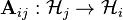
$\mathbf{A}_{ij} : \mathcal{H}_j \rightarrow \mathcal{H} _i$

is a bounded operator. If A is positive (semidefinite) in the sense that for all finite k and for any

$h \in \oplus _{n = 1 }^k \mathcal{H}_k ,$

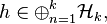
we have <h, Ah> ≥ 0, then there exists a lower triangular operator matrix L such that A = LL*. One can also take the diagonal entries of L to be positive.

[edit] See also

[edit] References

^ Press, William H.; Saul A. Teukolsky, William T. Vetterlink, Brian P. Flannery (1992). Numerical Recipes in C: The Art of Scientific Computing (second edition). Cambridge University Press. pp. 994. ISBN 0-521-43108-5. http://www.nr.com/.
^ D. Watkins, Fundamentals of Matrix Computations, p. 84

Bau III, David; Trefethen, Lloyd N. (1997), Numerical linear algebra, Philadelphia: Society for Industrial and Applied Mathematics, ISBN 978-0-89871-361-9 .
Gene H. Golub and Charles F. Van Loan, Matrix computations (3rd ed.), Section 4.2, Johns Hopkins University Press. ISBN 0-8018-5414-8.
Roger A. Horn and Charles R. Johnson. Matrix Analysis, Section 7.2. Cambridge University Press, 1985. ISBN 0-521-38632-2.
S. J. Julier and J.K. Uhlmann, "A new extension of the Kalman filter to nonlinear systems," in Proc. AeroSense: 11th Int. Symp. Aerospace/Defence Sensing, Simulation and Controls, 1997, pp. 182-193.

[edit] External links

[edit] Information

Cholesky Decomposition on PlanetMath
Cholesky Decomposition, The Data Analysis BriefBook
Module for Cholesky Factorization
Cholesky Decomposition on www.math-linux.com

[edit] Computer code

LAPACK is a collection of FORTRAN subroutines for solving dense linear algebra problems
ALGLIB includes a partial port of the LAPACK to C++, C#, Delphi, Visual Basic, etc.

[edit] Use of the matrix in simulation

[edit] Online calculators

Online Matrix Calculator Performs Cholesky decomposition of matrices online.

[0] Press, William H.; Saul A. Teukolsky, William T. Vetterlink, Brian P. Flannery (1992). Numerical Recipes in C: The Art of Scientific Computing (second edition). Cambridge University Press. pp. 994. ISBN 0-521-43108-5. http://www.nr.com/.

[1] D. Watkins, Fundamentals of Matrix Computations, p. 84

[1]

[2]