Logarithmic scale

From Wikipedia, the free encyclopedia

Various scales: lin-lin, lin-log, log-lin and log-log. Plotted graphs are: y = x (green), y = 10^x (red), y = log(x) (blue).

A logarithmic scale is a scale of measurement that uses the logarithm of a physical quantity instead of the quantity itself.

Presentation of data on a logarithmic scale can be helpful when the data covers a large range of values – the logarithm reduces this to a more manageable range. Some of our senses operate in a logarithmic fashion (Weber–Fechner law), which makes logarithmic scales for these input quantities especially appropriate. In particular our sense of hearing perceives equal ratios of frequencies as equal differences in pitch. In addition, studies of young children and an isolated tribe have shown logarithmic scales to be the most natural display of numbers by humans.^[1]

[edit] Definition and base

Logarithmic scales are either defined for ratios of the underlying quantity, or one has to agree to measure the quantity in fixed units. Deviating from these units means that the logarithmic measure will change by an additive constant. The base of the logarithm also has to be specified, unless the scale's value is considered to be a dimensional quantity expressed in generic (indefinite-base) logarithmic units.

[edit] Example scales

On most logarithmic scales, small values (or ratios) of the underlying quantity correspond to negative values of the logarithmic measure. Well-known examples of such scales are:

Richter magnitude scale and Moment magnitude scale (MMS) for strength of earthquakes and movement in the earth.
ban and deciban, for information or weight of evidence;
bel and decibel and neper for acoustic power (loudness) and electric power;
cent, minor second, major second, and octave for the relative pitch of notes in music;
logit for odds in statistics;
Palermo Technical Impact Hazard Scale;
Logarithmic timeline;
counting f-stops for ratios of photographic exposure;
rating low probabilities by the number of 'nines' in the decimal expansion of the probability of their not happening: for example, a system which will fail with a probability of 10^-5 is 99.999% reliable: "five nines".
Entropy in thermodynamics.
Information in information theory.
Particle Size Distribution curves of soil

Some logarithmic scales were designed such that large values (or ratios) of the underlying quantity correspond to small values of the logarithmic measure. Examples of such scales are:

pH for acidity;
stellar magnitude scale for brightness of stars;
Krumbein scale for particle size in geology.
Absorbance of light by transparent samples.

[edit] Logarithmic units

Logarithmic units are abstract mathematical units that can be used to express any quantities (physical or mathematical) that are defined on a logarithmic scale, that is, as being proportional to the value of a logarithm function. In this article, a given logarithmic unit will be denoted using the notation [log n], where n is a positive real number, and [log ] here denotes the indefinite logarithm function Log().

[edit] Examples

Examples of logarithmic units include common units of information and entropy, such as the bit [log 2] and the byte 8[log 2] = [log 256], also the nat [log e] and the ban [log 10]; units of relative signal strength magnitude such as the decibel 0.1[log 10] and bel [log 10], neper [log e], and other logarithmic-scale units such as the Richter scale point [log 10] or (more generally) the corresponding order-of-magnitude unit sometimes referred to as a factor of ten or decade (here meaning [log 10], not 10 years).

[edit] Motivation

The motivation behind the concept of logarithmic units is that defining a quantity on a logarithmic scale in terms of a logarithm to a specific base amounts to making a (totally arbitrary) choice of a unit of measurement for that quantity, one that corresponds to the specific (and equally arbitrary) logarithm base that was selected. Due to the identity $\log_b\,a = (\log_c\,a)/(\log_c\,b)$ , the logarithms of any given number a to two different bases (here b and c) differ only by the constant factor log_c b. This constant factor can be considered to represent the conversion factor for converting a numerical representation of the pure (indefinite) logarithmic quantity Log(a) from one arbitrary unit of measurement (the [log c] unit) to another (the [log b] unit), since

$\mathrm{Log}(a) = (\log_b\,a)[\log\,b] = (\log_c\,a)[\log\,c].$

For example, Boltzmann's standard definition of entropy S = k ln W (where W is the number of ways of arranging a system and k is Boltzmann's constant) can also written more simply as just S = Log(W), where "Log" here denotes the indefinite logarithm, and we let k = [log e]; that is, we identify the physical entropy unit k with the mathematical unit [log e]. This identity works because $\ln\,W = \log_e\,W = \mathrm{Log}(W)/[\log\,e]$ . Thus, we can interpret Boltzmann's constant as being simply the expression (in terms of more standard physical units) of the abstract logarithmic unit [log e] that is needed to convert the dimensionless pure-number quantity ln W (which uses an arbitrary choice of base, namely e) to the more fundamental pure logarithmic quantity Log(W), which implies no particular choice of base, and thus no particular choice of physical unit for measuring entropy.

[edit] Graphic representation

A log scale makes it easy to compare values which cover a large range, such as in this map

A logarithmic scale is also a graphical scale on one or both sides of a graph where a number x is printed at a distance c·log(x) from the point marked with the number 1. A slide rule has logarithmic scales, and nomograms often employ logarithmic scales. On a logarithmic scale an equal difference in order of magnitude is represented by an equal distance. The geometric mean of two numbers is midway between the numbers.

Logarithmic graph paper, before the advent of computer graphics, was a basic scientific tool. Plots on paper with one log scale can show up exponential laws, and on log-log paper power laws, as straight lines (see semilog graph, log-log graph).

[edit] Logarithmic and semi-logarithmic plots and equations of lines

Basically, log & semilog scales are best used to view two types of equations (for ease, the natural base 'e' is used):
(i) Y =exp(−aX)
(ii) Y = X^b
In the first case, plotting the equation on a semilog scale (log Y versus X) gives: log Y = −aX, which is linear.
In the second case, plotting the equation on a log-log scale (log Y versus log X) gives: log Y = b log X, which is linear.
When values that span large ranges need to be plotted, a logarithmic scale can provide a means of viewing the data that allows the values to be determined from the graph. The logarithmic scale is marked off in distances proportional to the logarithms of the values being represented. For example, in the figure below, for both plots, y has the values of: 1, 2, 3, 4, 5, 6, 7, 8, 9 10, 20, 30, 40, 50, 60, 70, 80, 90 and 100. For the plot on the left, the log₁₀ of the values of y are plotted on a linear scale. Thus the first value is log₁₀(1) = 0; the second value is log₁₀(2) = 0.301; the 3rd value is log₁₀(3) = 0.4771; the 4th value is log₁₀(4) = 0.602, and so on. The plot on the right uses logarithmic (or log, as it is also referred to) scaling on the vertical axis. Note that values where the exponent term is close to an integral fraction of 10 (0.1, 0.2, 0.3, etc) are shown as 10 raised to the power that yields the original value of y. These are shown for y = 2, 4, 8, 10, 20, 40, 80 and 100.

Plots of the log (base 10) of values of y (see text) on a linear scale (left plot) and of values of y on a log scale (right plot).

Note that for y = 2 and 20, y = 10^0.301 and 10^1.301; for y = 4 and 40, y = 10^0.602 and 10^1.602. This is due to the law that

$\log(AB) = \log(A) + \log(B).\,$

So, knowing log₁₀(2) = 0.301, the rest can be derived:

log₁₀(4) = log₁₀(2 × 2) = log₁₀(2) + log₁₀(2) = 0.602

log₁₀(20) = log₁₀(2 × 10) = log₁₀(2) + log₁₀(10) = 1.301

Note that the values of y are easily picked off the above figure. By comparison, values of y less than 10 are difficult to determine from the figure below, where they are plotted on a linear scale, thus confirming the earlier assertion that values spanning large ranges are more easily read from a logarithmically scaled graph.

Plot of the values of y (see text) on a linear scale.

[edit] Log-log plots

If both the vertical and horizontal axis of a plot is scaled logarithmically, the plot is referred to as a log-log plot. The equation for a line on a log-log scale would be:

log(F(x)) = m log(x) + b,

F(x) = (x^m)(10^b),

where m is the slope and b is the intercept point on the log plot. The example plot shown below is for the equation log(F(x)) = m log(x) + b, for m = −10, b = 20.

Plot on log-log scale of equation F(x) = (x⁻¹⁰ )(10²⁰).

[edit] Slope of a log-log plot

Finding the slope of a log-log plot using ratios

To find the slope of the plot, two points are selected on the x-axis, say x₁ and x₂. Using the above equation:

$\mathrm {log}[F (x_1)] = m\ \mathrm{log}(x_1) + b \ ,$

and

$\mathrm {log}[F (x_2)] = m\ \mathrm{log}(x_2) + b \ .$

The slope m is found taking the difference:

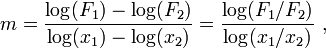
$m = \frac { \mathrm {log} (F_1) - \mathrm {log} (F_2)} { \mathrm{log}(x_1) - \mathrm{log}(x_2) } = \frac {\mathrm {log} (F_1/F_2)}{\mathrm{log}(x_1/x_2)} \ ,$

where F₁ is shorthand for F ( x₁ ) and the same for F₂. The figure at right illustrates the formula. Notice that the slope in the example of the figure is negative. The formula also provides a negative slope, as can be seen from the following property of the logarithm:

$\mathrm{log}(x_1/x_2) = -\mathrm{log}(x_2/x_1) \ .$

[edit] Finding the function from the log-log plot

The above procedure now is reversed to find the form of the function F(x) using its (assumed) known log-log plot. To find the function F, pick some fixed point (x₀, F₀), where F₀ is shorthand for F( x ₀), somewhere on the straight line in the above graph, and further some other arbitrary point (x, F) on the same graph. Then from the slope formula above:

$m = \frac {\mathrm {log} (F/F_0)}{\mathrm{log}(x/x_0)}$

which leads to

$\mathrm{log}(F / F_0) = m \,\, \mathrm{log}(x / x_0) = \mathrm{log}[(x / x_0)^m ]\ .$

Notice that 10^{log₁₀( F )} = F . Therefore, the logs can be inverted to find:

$\frac{F}{F_0} = (\frac{x}{x_0})^m$

or

$F = \frac{F_0}{(x_0)^m} \,\, x^m$ ,

which means that

$F = \mathrm{const}\,\, x^m$

In other words, F is proportional to x to the power of the slope of the straight line of its log-log graph. Of course, the inverse is true too: any function of the form

$F = \mathrm{const} \,\, x^m$

will have a straight line as its log-log graph representation, where the slope of the line is ‘’m’’.

[edit] Semi logarithmic plots

If only the ordinate or abscissa is scaled logarithmically, the plot is referred to as a semi logarithmic plot. The equation for a line with an ordinate axis logarithmically scaled would be:

log(F(x)) = mx + b

F(x) = 10^{(mx + b)} = (10^mx)(10^b)

The equation of a line on a plot where the abscissa axis is scaled logarithmically would be

F(x) = m log₁₀(x) + b.

[edit] Estimating values in a diagram with logarithmic scale

One method for accurate determination of values on a logarithmic axis is as follows:

Measure the distance from the point on the scale to the closest decade line with lower value with a ruler.
Divide this distance by the length of a decade (the length between two decade lines).
The value of your chosen point is now the value of the nearest decade line with lower value times 10^a where a is the value found in step 2.

Example: What is the value that lies halfway between the 10 and 100 decades on a logarithmic axis? Since it is the halfway point that is of interest, the quotient of steps 1 and 2 is 0.5. The nearest decade line with lower value is 10, so the halfway point's value is (10^0.5) × 10 = 10^1.5 ≈ 31.62.

To estimate where a value lies within a decade on a logarithmic axis, use the following method:

Measure the distance between consecutive decades with a ruler. You can use any units provided that you are consistent.
Take the log (value of interest/nearest lower value decade) multiplied by the number determined in step one.
Using the same units as in step 1, count as many units as resulted from step 2, starting at the lower decade.

Example: To determine where 17 is located on a logarithmic axis, first use a ruler to measure the distance between 10 and 100. If the measurement is 30mm on a ruler (it can vary — ensure that the same scale is used throughout the rest of the process).

[log (17/10)] × 30 = 6.9

x = 17 is then 6.9mm after x = 10 (along the x-axis).

[edit] Logarithmic interpolation

Interpolating logarithmic values is very similar to interpolating linear values. In linear interpolation, values are determined through equal ratios. For example, in linear interpolation, a line that increases one ordinate (y-value) for every two abscissa (x-value) has a ratio (also known as slope or rise-over-run) of 1/2. In order to determine the ordinate or abscissa of a particular point, you must know the other value. The calculation of the ordinate corresponding to an abscissa of 12 in the example below is as follows:

1/2 = Y/12

Y is the unknown ordinate. Using cross-multiplication, Y can be calculated and is equal to 6.

In logarithmic interpolation, a ratio of logarithmic values is set equal to a ratio of linear values. For example, consider a log base 10 scale graph of paper reams sold per day measuring 19 1/32nds of an inch from 1 to 10. How many reams were sold in a day if the value on the graph is 11 1/32nds between 1 and 10? In order to solve this problem, it is necessary to use a basic logarithmic definition:

log(A) - log(B) = log(A/B)

Decade lines, those values that denote powers of the log base, are also important in logarithmic interpolation. Locate the lower decade line. It is the closest decade line to the number you are evaluating that is lower than that number. Decade lines begin at 1. The next decade line is the first power of your log base. For log base 10, the first decade line is 1, the second is 10, the third is 100, and so on.

The ratio of linear values is the number of units from the lower decade line to the value of interest (11 1/32nds in this example, since the lower decade line in this example is 1) divided by the total number of units between the lower decade line and the upper decade line (the upper decade line is 10 in this example). Therefore, the linear ratio is:

11/19

Notice that the units (1/32nds of an inch) are removed from the equation because both measurements are in the same units. Conversion to a single unit before calculating the ratio is required if the measurements were made in different units.

The logarithmic ratio uses the same graphical measurements as the linear ratio. The difference between the log of the upper decade line (10) and the log of the lower decade line (1) represents the same graphical distance as the total number of units between the two decade lines in the linear ratio (19 1/32nds of an inch). Therefore, the lower part of the logarithmic ratio (the bottom part of the fraction) is:

log(10) - log(1)

The upper part of the logarithmic ratio (the top part of the fraction) represents the same graphical distance as the number of units between the value of interest (number of reams of paper sold) and the lower decade line in linear ratio (11 1/32nds of an inch). The unknown in this ratio is the value of interest, which we will define as "X". Therefore, the top part of the fraction is:

log(X) - log(1)

The logarithmic ratio is:

[log(X) - log(1)]/[log(10) - log(1)]

The linear ratio is equal to the logarithmic ratio. Therefore, the equation required to determine the number of paper reams sold in a particular day is:

11/19 = [log(X) - log(1)]/[log(10) - log(1)]

This equation can be rewritten using the logarithmic definition mentioned above:

11/19 = log(X/1)/log(10)

log(10) = 1, therefore:

11/19 = log(X/1)

In order to remove the "log" from the right side of the equation, both sides must be used as exponents for the number 10, meaning 10 to the power of 11/19 and 10 to the power of log(X/1). The "log" function and the "10 to the power of" function are reciprocal and cancel each other out, leaving:

10^(11/19) = X/1

Now both sides must be multiplied by 1. While the 1 drops out of this equation, it is important to note that the number X is divided by is the value of the lower decade line. If this example involved values between 10 and 100, the equation would include "X/10" instead of "X/1".

10^(11/19) = X

X = 3.793 reams of paper.

[edit] References

^ "Slide Rule Sense: Amazonian Indigenous Culture Demonstrates Universal Mapping Of Number Onto Space". ScienceDaily. 2008-05-30. http://www.sciencedaily.com/releases/2008/05/080529141344.htm. Retrieved on 2008-05-31.
which references: Stanislas, Dehaene; Véronique Izard, Elizabeth Spelke, and Pierre Pica. (2008). "Log or Linear? Distinct Intuitions of the Number Scale in Western and Amazonian Indigene Cultures". Science 320 (5880): 1217. doi:10.1126/science.1156540. PMID 18511690.

[edit] See also

Mathematics portal

[edit] Units of information

bit [log 2]
byte 8[log 2] = [log 256]
nat [log e]
ban [log 10]

[edit] Units of relative signal strength

bel [log 10]
decibel 0.1[log 10]
neper [log e]

[edit] Scale

[edit] Applications

[edit] External links

Height - an issue of xkcd drawn on a logarithmic scale

Wikimedia Commons has media related to: Logarithmic scale

[0] "Slide Rule Sense: Amazonian Indigenous Culture Demonstrates Universal Mapping Of Number Onto Space". ScienceDaily. 2008-05-30. http://www.sciencedaily.com/releases/2008/05/080529141344.htm. Retrieved on 2008-05-31.
which references: Stanislas, Dehaene; Véronique Izard, Elizabeth Spelke, and Pierre Pica. (2008). "Log or Linear? Distinct Intuitions of the Number Scale in Western and Amazonian Indigene Cultures". Science 320 (5880): 1217. doi:10.1126/science.1156540. PMID 18511690.

[1]